Lab 5: Resource Selection
Elie Gurarie
Loading important packages for later:
pcks <- list("plyr", "lubridate", "rgdal", "sp", "raster", "magrittr")
sapply(pcks, require, char = TRUE)
## [1] TRUE TRUE TRUE TRUE TRUE TRUELoad movement and habitat data:
load("./_data/caribou.rda")
load("./_data/habitat.rda")
1 Central resource selection question
For now, it is: What elevations and what landcovers do different herds prefer, in different seasons?
Recall our plotting code (from the Spatial Lab)
plot(elevation)
image(landcover, col = landcover.legend$Color, asp = 1)
with(na.omit(landcover.legend), legend("bottomleft", fill = Color, legend = Type,
    cex = 0.6, ncol = 2, bg = "white"))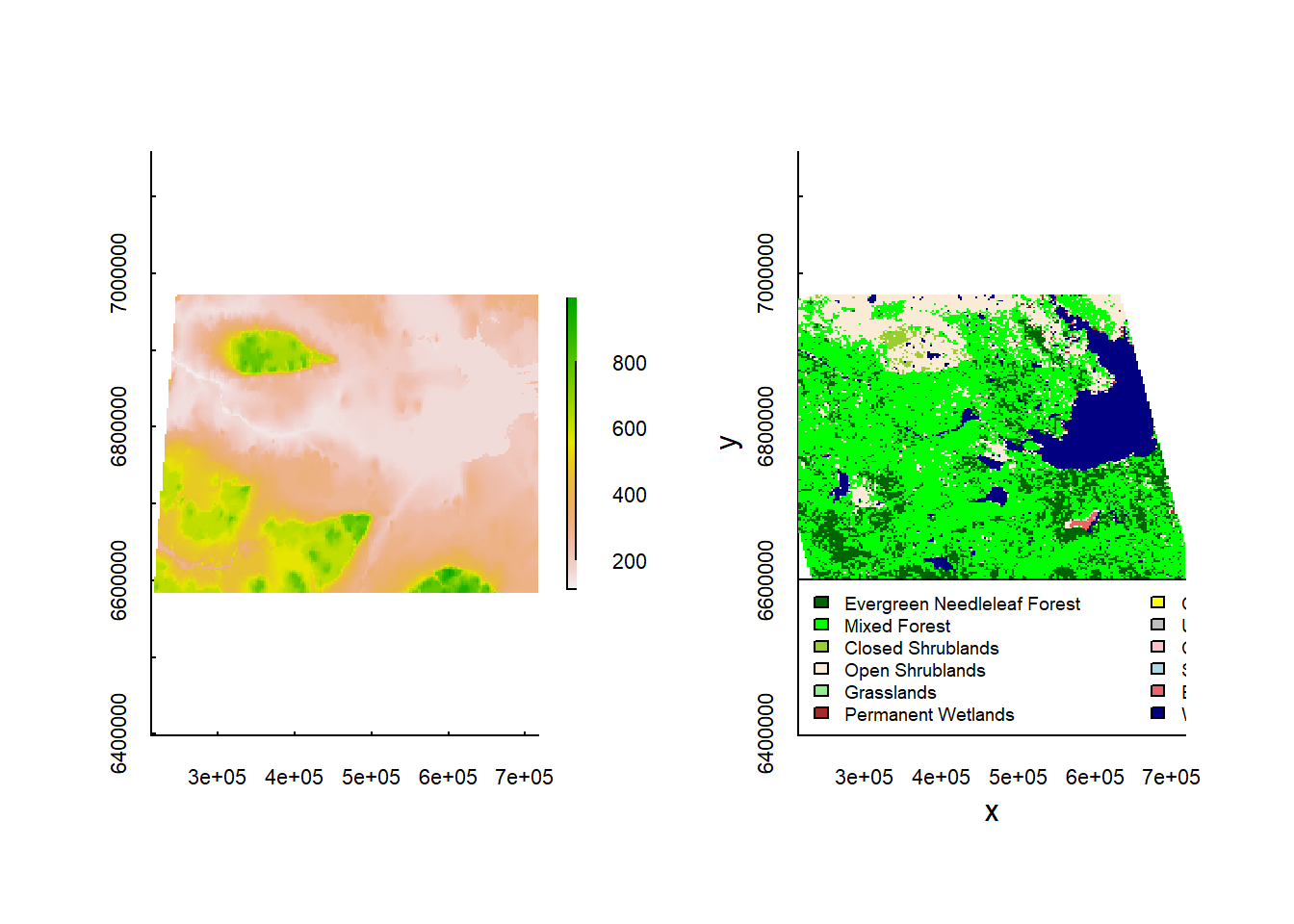
1.1 Simplifying the landcover data
Note that in the landcover data, there are several landscape types that are hardly represented:
table(landcover@data@values)##
## 1 5 6 7 10 11 12 14 15 16 17
## 5363 16619 234 4045 4 82 2 81 2 64 3411The landcover legend contains their interpretation:
values <- landcover@data@values
Type <- landcover.legend$Type[values]
merge(landcover.legend, as.data.frame(table(Type))) %>% arrange(Value)
## Type Value Color Freq
## 1 Evergreen Needleleaf Forest 1 darkgreen 5363
## 2 Evergreen Broadleaf Forest 2 <NA> 0
## 3 Deciduous Needleleaf Forest 3 <NA> 0
## 4 Deciduous Broadleaf Forest 4 <NA> 0
## 5 Mixed Forest 5 green 16619
## 6 Closed Shrublands 6 yellowgreen 234
## 7 Open Shrublands 7 antiquewhite 4045
## 8 Woody Savannas 8 <NA> 0
## 9 Savannas 9 <NA> 0
## 10 Grasslands 10 lightgreen 4
## 11 Permanent Wetlands 11 brown 82
## 12 Croplands 12 yellow 2
## 13 Urban and Built-Up 13 grey 0
## 14 Cropland/Natural Vegetation Mosaic 14 pink 81
## 15 Snow and Ice 15 lightblue 2
## 16 Barren or Sparsely Vegetated 16 indianred2 64
## 17 Water Bodies 17 navy 3411Basically, everything from 10 to 16 is negligible. We can pool them all into “other”, and perhaps also pool Closed and Open Shrublands into a single category.
Type.new <- as.character(Type)
Type.new[values %in% 8:16] <- "Other"
Type.new[values %in% 6:7] <- "Shrubland"
Type.new <- factor(Type.new)
levels(Type.new)
## [1] "Evergreen Needleleaf Forest" "Mixed Forest"
## [3] "Other" "Shrubland"
## [5] "Water Bodies"Now that we have a new simplified assignments, lets create a simplified landcover, which is identical, except it contains differeng values:
landcover.new <- landcover
landcover.new@data@values <- as.integer(Type.new)
cols.new <- c("darkgreen", "green", "grey", "yellow", "blue")
image(landcover.new, col = cols.new, asp = 1)
legend("bottomleft", fill = cols.new, legend = levels(Type.new), cex = 0.8)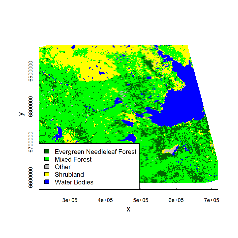
Okay, now we have a simplified landcover raster.
2 Estimating a resource selection function
Assuming that some habitats are actively preferred (or selected) over other habitats, the RSF attempts to quantify that preference (or avoidance). The strategy is simple: - Collect data on used locations - Define and collect data on available (but not used) locations - Perform a logistic regression
The RSF itself looks like: \[w(X) = \exp(\beta_1 x_1 + \beta_2 x_2 + \beta_3 x_3 + ...)\] Where positive \(\beta\)’s correspond to a preference score and negative \(\beta\)’s correspond to avoidance.
2.1 Availability
Perhaps the trickiest part of this is defining “availability”. A common thing to do is exactly what we did in the exploratory analysis lab, which is draw an MCP and draw random points from within it. Lets do this for the MacKenzie herd:
require(adehabitatHR)
load("./_data/caribou.daily.rda")
MK <- subset(caribou.daily, Herd == "Mackenzie")
MK.sp <- SpatialPoints(MK[, c("X", "Y")])
MK.landcover <- crop(landcover.new, extent(MK.sp))
MK.elevation <- crop(elevation, extent(MK.sp))
# plot elevations and line
image(MK.landcover, asp = 1, col = cols.new)
with(MK, points(X, Y, type = "o", pch = 19, cex = 0.5, col = rgb(0, 0, 0, 0.2)))

# compute mcp
MK.mcp <- mcp(MK.sp, 100)
lines(MK.mcp, col = "red", lwd = 2)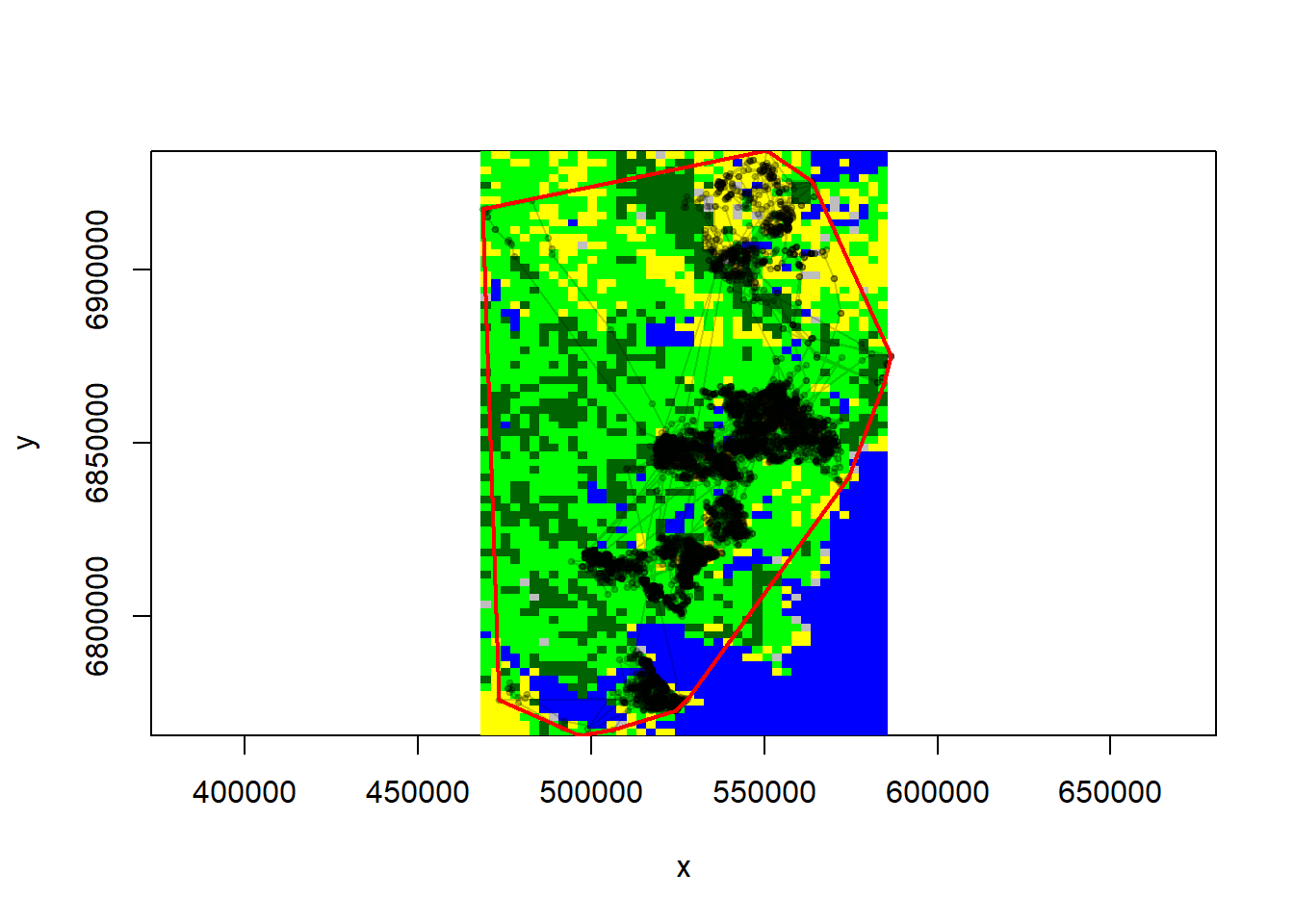
Now obtain some random points from within the MCP. You should get a number comparable to the number of observations (often larger, but with a dataset this large it doesn’t matter too much). In fact, we should subsample the total movement data set - in an ad hoc battle against autocorrelations:
xy.obs <- MK[sample(1:nrow(MK), 1000), c("X", "Y")]
xy.random <- spsample(MK.mcp, 1000, "random")@coords
plot(xy.random, asp = 1, col = "darkblue", pch = 19, cex = 0.5)
points(xy.obs, pch = 19, col = rgb(1, 1, 0, 0.4), cex = 0.5)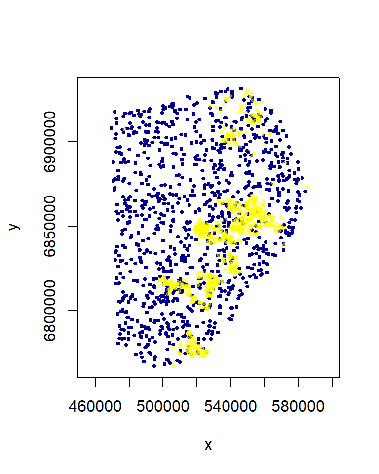
We stack the used and available “observations”, and label them and Used: TRUE/FALSE:
Data.rsf <- data.frame(X = c(xy.obs[, 1], xy.random[, 1]), Y = c(xy.obs[, 2],
    xy.random[, 2]), Used = c(rep(TRUE, nrow(xy.obs)), rep(FALSE, nrow(xy.random))))
Now, we extract the two variables we have for the real and random observations:
Data.rsf$elevation <- raster::extract(elevation, Data.rsf[, 1:2])
Data.rsf$landcover <- raster::extract(landcover.new, Data.rsf[, 1:2])
Data.rsf$landtype <- levels(Type.new)[Data.rsf$landcover]
head(Data.rsf)
## X Y Used elevation landcover landtype
## 1 525388.5 6849817 TRUE 197 2 Mixed Forest
## 2 546363.5 6848355 TRUE 223 2 Mixed Forest
## 3 517409.3 6805346 TRUE 159 2 Mixed Forest
## 4 523208.0 6848394 TRUE 189 2 Mixed Forest
## 5 521228.5 6847762 TRUE 188 2 Mixed Forest
## 6 543959.8 6864145 TRUE 232 2 Mixed Forest2.2 Visually compare used and observed
boxplot(elevation ~ Used, data = Data.rsf)
mosaicplot(landtype ~ Used, data = Data.rsf, shade = TRUE)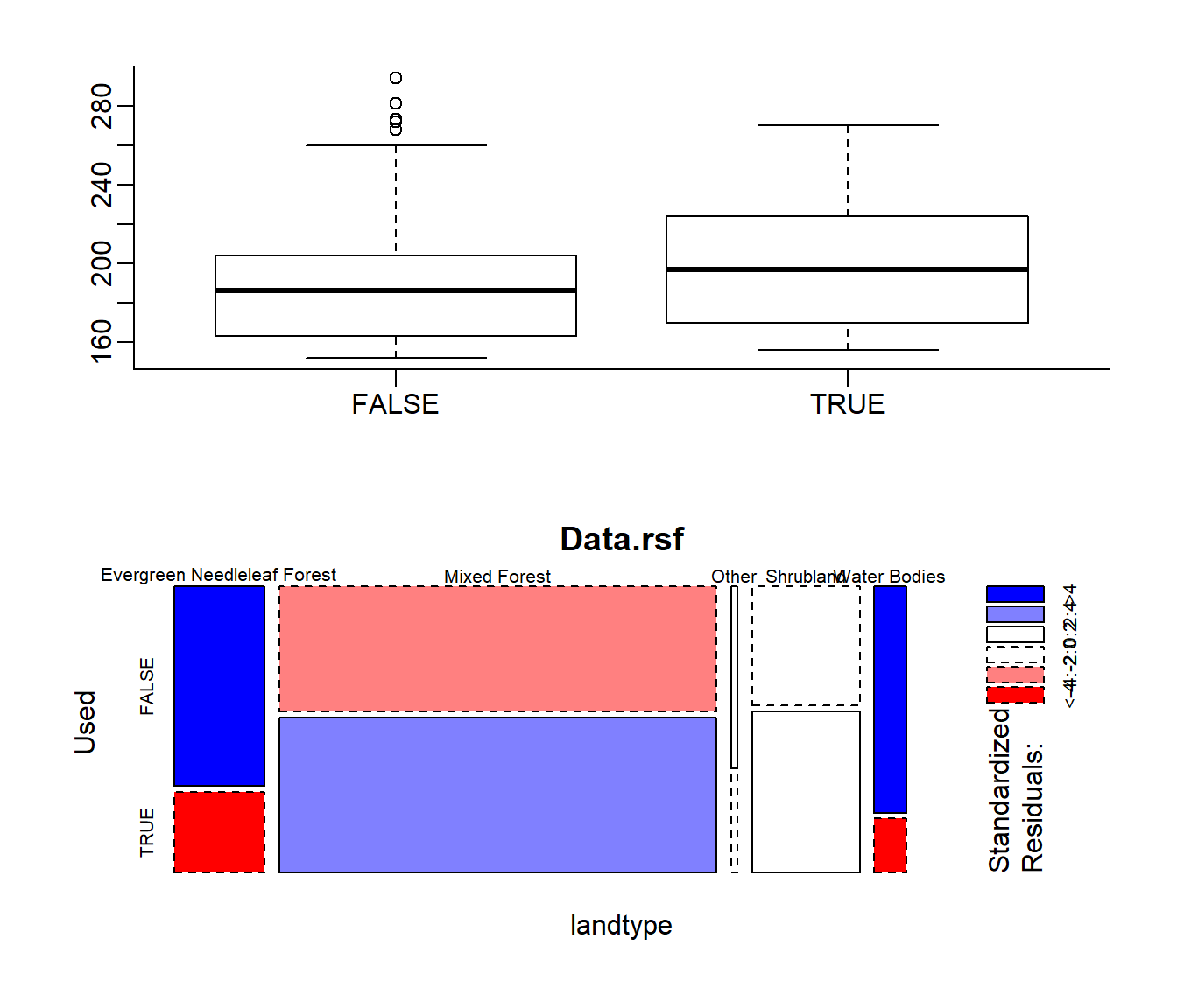
The blue and red colors represent prefernces and avoidances, respectively, in the mosaic plot.
2.3 Fit an rsf
Easy as performing a glm:
RSF.fit <- glm(Used ~ scale(elevation) * (landtype - 1), data = Data.rsf, family = "binomial")Looks like a good model! A quick way to plot coefficietns:
library(sjPlot)
plot_model(RSF.fit)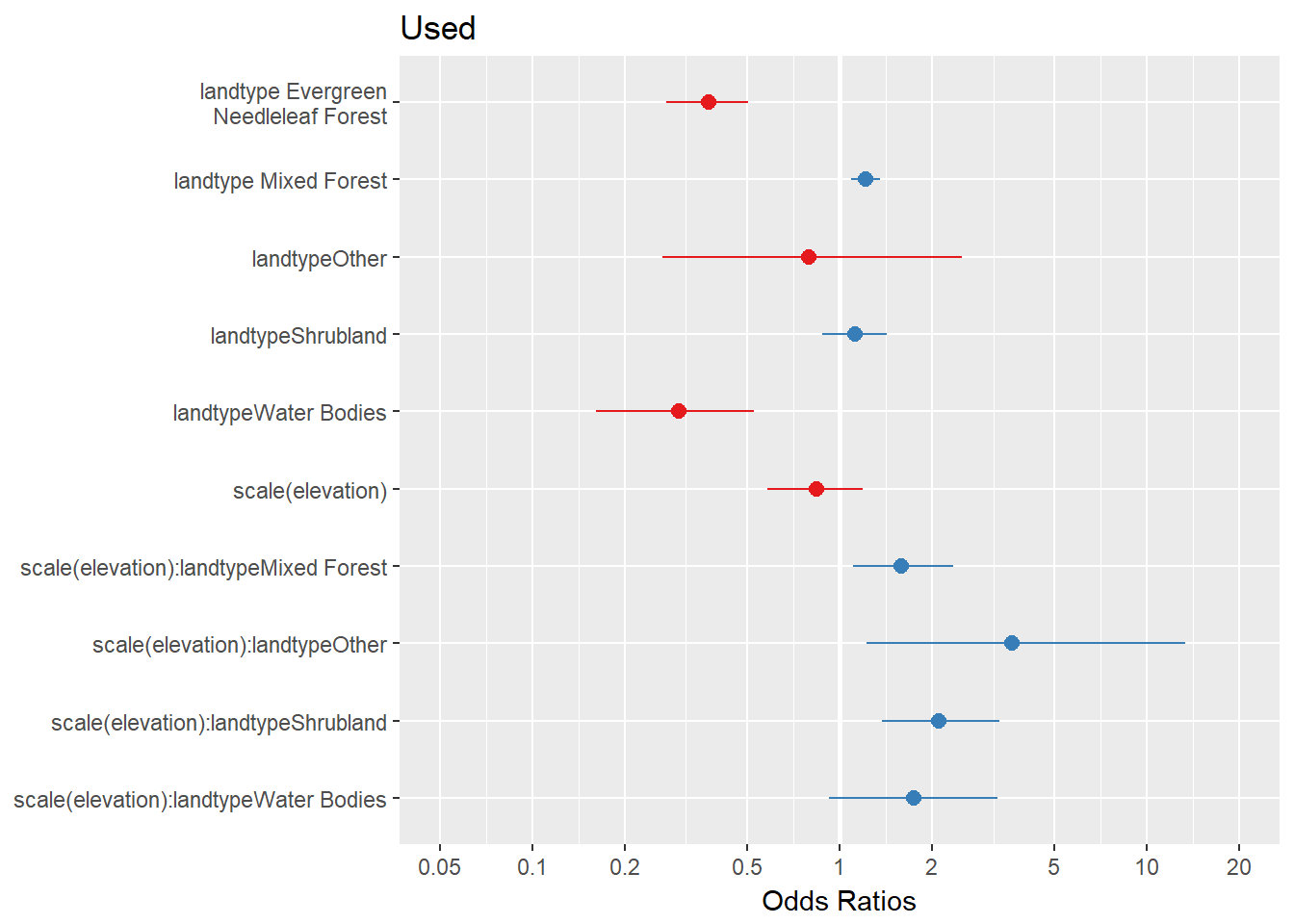
2.4 RSF prediction
Make sure we have prediction scopes that match:
MK.landcover <- crop(landcover.new, extent(MK.sp))
MK.elevation <- crop(elevation, extent(MK.sp))
MK.rsf <- MK.elevation
Extract the approporiate vectors:
MK.landtype.vector <- levels(Type.new)[MK.landcover@data@values]
MK.elevation.vector <- MK.elevation@data@values
Predict.df <- data.frame(landtype = MK.landtype.vector, elevation = MK.elevation.vector)
THe key little function is predict (with newdata):
MK.rsf@data@values <- predict(RSF.fit, newdata = Predict.df)Plot the results:
plot(MK.elevation, main = "elevation")
plot(MK.landcover, col = cols.new, main = "landcover")
plot(MK.rsf, main = "rsf", col = grey.colors(100, start = 0, end = 1))
points(MK[, c("X", "Y")], col = alpha("yellow", 0.01), cex = 0.5)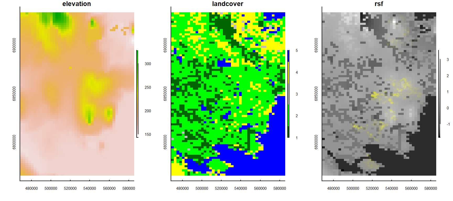
Of course … this barely scratches the surface! It is just the basic technique to adapt to answer all kinds of interesting questions.