Lab 3: Loading and Plotting Spatial Data
Elie Gurarie
1 Background
Animals live and move in structured, heterogeneous space. Most analyses of movement are not limited to describing the properties of displacement, but ask some questions with respect to spatial variables. Spatial data objects in R can be rather complex - broadly, a landscape can be described in terms of vectors, which include polygons (e.g. - boundaries of a projected area), lines (e.g. roads), points (e.g. houses) or in terms of a raster which is just a grid (usually square) where each cell has a particular value, whether discrete (e.g. a land-cover type) or continuous (e.g. an elevation).
There are some packages that are very helpful for working with raster and spatial data. Here’s a list, in approximate decreasing order of usefulness:
spprovides the classes for spatial data; makes coordinate transformations simplerastergeneral-purpose raster functions; reads raster objects into R (very fast)rgdalreads shape files into Rrgeosa collection of excellent methods for working with spatial objectsspatstatnitty-gritty spatial calculations in compiled C code; model-fittingadehabitatHRtools for home range estimation, such as 95% MCPmaptoolsconversion between spatstat and spatial objectsadehabitatMAfunctions that make it easier to work rastersmapdataa collection of map databases, though you might find higher-resolution maps elsewhere
In this lab, we will:
- Load line and polygon shape files
- Load raster files of land cover types and elevation
- Practice projecting into consistent coordinate systems and plotting
Note: An absolutely awesome, detailed tutorial on these topics can be found here: http://rspatial.org/spatial/index.html
2 Shape files
From Wikipedia: The shapefile format is a popular geospatial vector data format for geographic information system (GIS) software. It is developed and regulated by Esri as a (mostly) open specification for data interoperability among Esri and other GIS software products. In practice, is is actually several files, all of which have the same name and the following extentions:
.shp— shape format; the feature geometry itself.shx— shape index format; a positional index of the feature geometry to allow seeking forwards and backwards quickly.dbf— attribute format; columnar attributes for each shape, in dBase IV format.prj— projection format; the coordinate system and projection information, a plain text file describing the projection using well-known text format.
(NB: This list is not complete - see the Wikipedia page).
2.1 Polygon: National Park Boundary
You can download shape files for any protected area on earth from https://www.protectedplanet.net, including Wood Buffalo National Park in Canada (click link for source of shape file).
We downloaded and renamed this file and placed them in the habitatdata.zip file here: https://terpconnect.umd.edu/~egurarie/teaching/SpatialModelling_NWT2018/data/ You can download the file, and copy the entire WoodBuffaloNP folder somewhere useful on your computer. Shape files are loaded with the readOGR command.
require(rgdal)
wbnp <- readOGR("./_data/WoodBuffaloNP")
## OGR data source with driver: ESRI Shapefile
## Source: "./_data/WoodBuffaloNP", layer: "WDPA_Mar2018_protected_area_611-shapefile-polygons"
## with 1 features
## It has 28 fields
## Integer64 fields read as strings: STATUS_YR METADATAIDplot(wbnp, main = "Wood Buffalo N.P.", axes = TRUE, col = "green")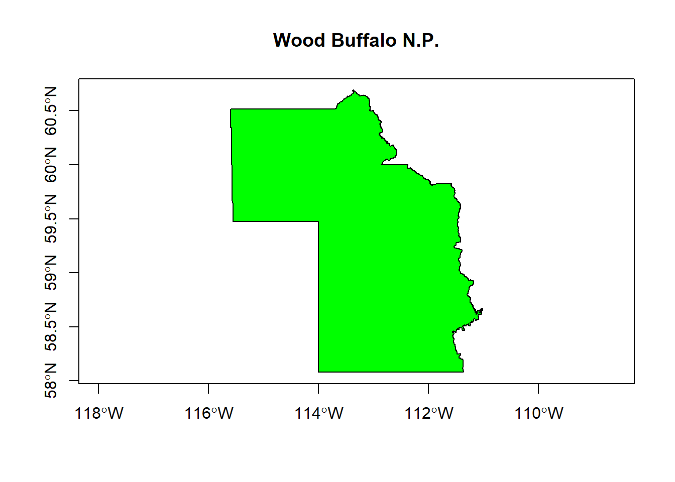
Note, wbnp is an exotic object called a SpatialPolygonsDataFrame, which contains a lot of important spatial information but (in this case) just one set of coordinates for a single polygon. Important features of this object include:
- The polygon information (only one row!)
wbnp@data## WDPAID WDPA_PID PA_DEF NAME
## 0 611 611 1 Wood Buffalo National Park of Canada
## ORIG_NAME DESIG
## 0 Wood Buffalo National Park of Canada National Park of Canada
## DESIG_ENG DESIG_TYPE IUCN_CAT INT_CRIT MARINE
## 0 National Park of Canada National II Not Applicable 0
## REP_M_AREA GIS_M_AREA REP_AREA GIS_AREA NO_TAKE NO_TK_AREA
## 0 0 0 35832 45352.47 Not Applicable 0
## STATUS STATUS_YR GOV_TYPE OWN_TYPE
## 0 Designated 1922 Federal or national ministry or agency State
## MANG_AUTH
## 0 Government of Canada, Parks Canada Agency
## MANG_PLAN VERIF METADATAID SUB_LOC
## 0 http://www.pc.gc.ca/index_e.asp State Verified 1868 CA-AB;CA-NT
## PARENT_ISO ISO3
## 0 CAN CAN- the projection
wbnp@proj4string## CRS arguments:
## +proj=longlat +datum=WGS84 +no_defs +ellps=WGS84 +towgs84=0,0,0- the boundary box
bbox(wbnp)## min max
## x -115.60311 -111.01704
## y 58.07851 60.69092- the coordinates of the one polygon (very tedious!)
wbnp.ll <- wbnp@polygons[[1]]@Polygons[[1]]@coordsA quick ggmap of the park boundaries:
require(ggmap)
require(scales)
mymap <- get_map(bbox(wbnp), maptype = "terrain", zoom = 7)
ggmap(mymap) + geom_polygon(data = data.frame(wbnp.ll), aes(x = X1, y = X2),
    fill = alpha("pink", 0.2), col = "darkred")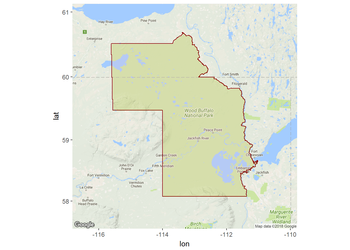
Now that we have the park boundaries, we can load our caribou object and see which of the caribou are in the park:
load("./_data/caribou.rda")
parkmap <- ggmap(mymap) + geom_polygon(data = data.frame(wbnp.ll), aes(x = X1,
    y = X2), fill = alpha("pink", 0.2), col = "darkred")
parkmap + geom_point(data = caribou, aes(x = Longitude, y = Latitude, col = Herd),
    alpha = 0.5)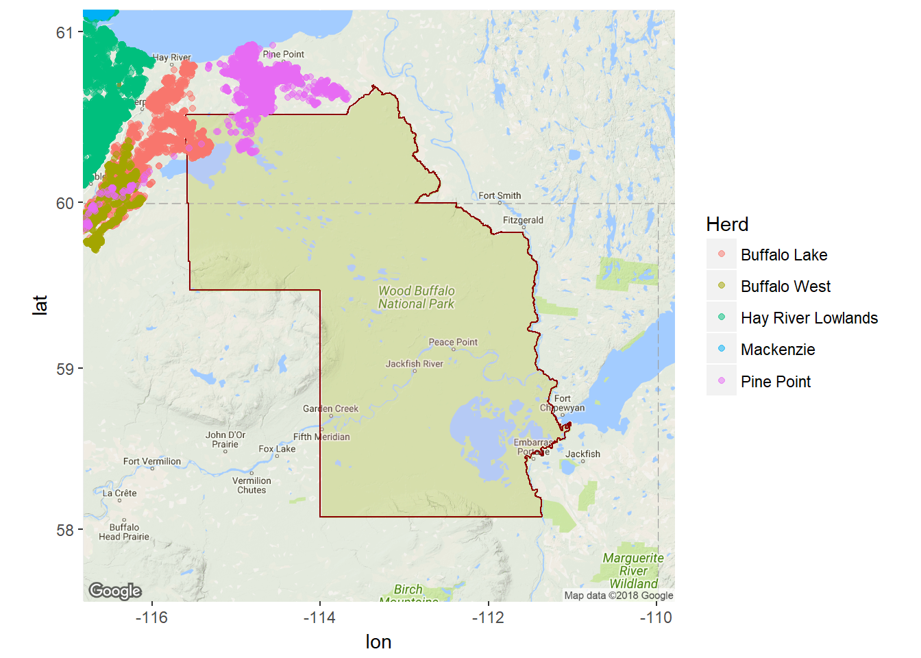
Ok - not too many animals enter the protected area, but at least it was easy to find that out!
2.2 Lines: Human development
Here, we load a shape file that consists of a bunch of linear elements around the South Slave Boreal. Download and unpack the lines2010 files into a folder and use readORG to load it:
directory <- "./_data/lines2010"
lines2010 <- readOGR(directory)
## OGR data source with driver: ESRI Shapefile
## Source: "./_data/lines2010", layer: "lines2010"
## with 19075 features
## It has 3 fieldsThis step will take a little while - with a message that it’s working. A quick look at the summary and a plot gives us some idea of the data:
summary(lines2010)## Object of class SpatialLinesDataFrame
## Coordinates:
## min max
## x -1398160 -931815.2
## y 2295440 2798279.4
## Is projected: TRUE
## proj4string :
## [+proj=lcc +lat_1=50 +lat_2=70 +lat_0=40 +lon_0=-96 +x_0=0 +y_0=0
## +datum=NAD83 +units=m +no_defs +ellps=GRS80 +towgs84=0,0,0]
## Data attributes:
## Herd Class Province
## Bistcho :9854 Airstrip : 17 Alberta :11173
## Caribou Mountain : 278 Pipeline : 443 NorthWestTerritories: 7902
## FortSmith : 1 Powerline: 134
## North_West : 2 Railway : 31
## NorthWestAlberta1: 9 Road : 1225
## NWT :7899 Seismic :17218
## Yates :1032 Unknown : 7Note that there are 7 “classes” to the data. We can get their names from the @data slot:
classes <- levels(lines2010@data$Class)And we can plot the data, color coded by class as follows:
plot(lines2010, col = lines2010@data$Class)
legend("topright", legend = classes, col = 1:length(classes), lty = 1, bty = "n")
axis(1)
axis(2)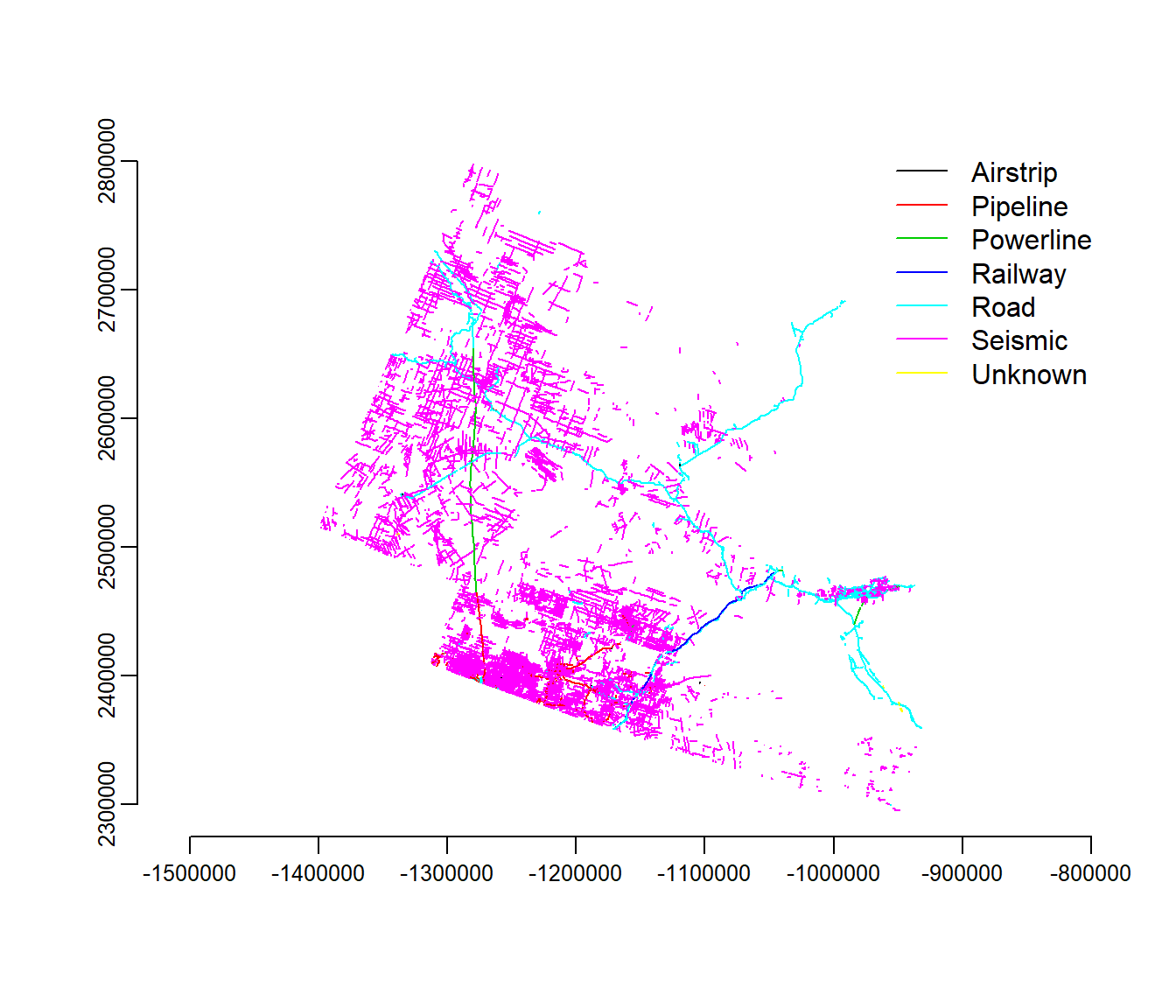
2.3 Re-projecting
Note that these data are definitely not in lat-long. The projection is:
require(raster)
projection(lines2010)
## [1] "+proj=lcc +lat_1=50 +lat_2=70 +lat_0=40 +lon_0=-96 +x_0=0 +y_0=0 +datum=NAD83 +units=m +no_defs +ellps=GRS80 +towgs84=0,0,0"Which is the proj4 code for the Canadian Lambert Conic. Let’s reproject the data into of our caribou data, which (remember) we stored when we saved it.
load("./_data/caribou.rda")
(utm11.proj4 <- attr(caribou, "projection"))
## [1] "+proj=utm +zone=11 +ellps=GRS80 +towgs84=0,0,0,0,0,0,0 +units=m +no_defs"The command that performs the projection on spatial objects is spTransform. Minor note: the projection has be to a CRS (Coordinate Reference System) type object, generated with the crs() function.
lines2010.utm <- spTransform(lines2010, crs(utm11.proj4))Now we can plot the lines data and the caribou data on the same figure. In the figure below, I went through the effort of making the color coding more attractive.
load("./_data/caribou.rda")

classes <- levels(lines2010.utm@data$Class)
legend.args <- data.frame(classes, col = c("blue", "brown", "red", "green",
    "black", "lightgrey", "white"), lty = c(1, 1, 2, 3, 1, 1, 1), lwd = c(2,
    3, 2, 2, 1.5, 1, 1))

plot(lines2010.utm, col = as.character(legend.args$col[lines2010.utm$Class]),
    lty = legend.args$lty[lines2010.utm$Class], lwd = legend.args$lwd[lines2010.utm$Class])

with(legend.args[-7, ], legend("bottomleft", ncol = 1, col = as.character(col),
    lty = lty, lwd = lwd, legend = classes, bty = "n", cex = 0.8, title = "linear elements"))

require(gplots)
require(scales)
n.herds <- length(unique(caribou$Herd))
palette(rich.colors(n.herds))
with(caribou[seq(1, nrow(caribou), 10), ], points(X, Y, col = alpha(as.integer(Herd),
    0.2), pch = 19, cex = 0.5))

legend("topright", ncol = 1, bty = "n", col = 1:n.herds, pch = 19, legend = levels(caribou$Herd),
    cex = 0.8, title = "boreal caribou herds")

axis(1)
axis(2)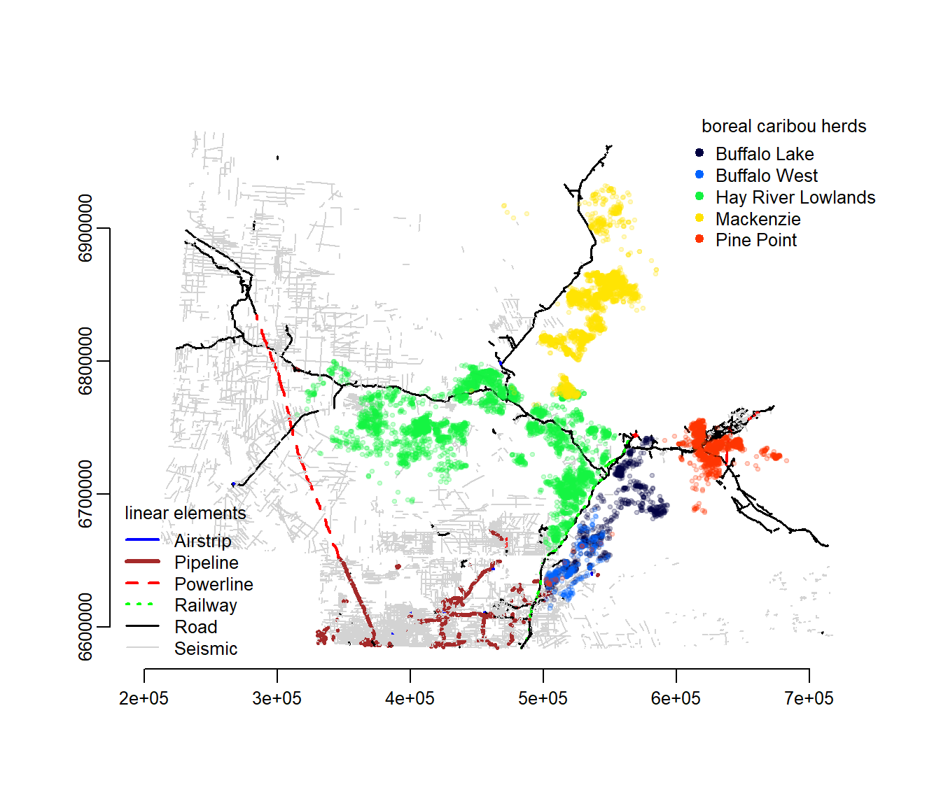
3 Rasters
3.1 Continuous: Digital Elevation
Rasters are very efficient spatial matrices. They break up space into equal sized grids and store attributes at each grid point. One common way they are stored is as geoTiff objects. This link: https://TBD should contain several rasters, notably elevation.tif - a digital elevation model. I downloaded this dataset (called: GTOPO30) from the excellent USGS Earth Explorer data page here: https://earthexplorer.usgs.gov/. Download elevation.tif to your data drive and load them, with the raster command:
elevation <- raster("./_data/elevation.tif")
plot(elevation)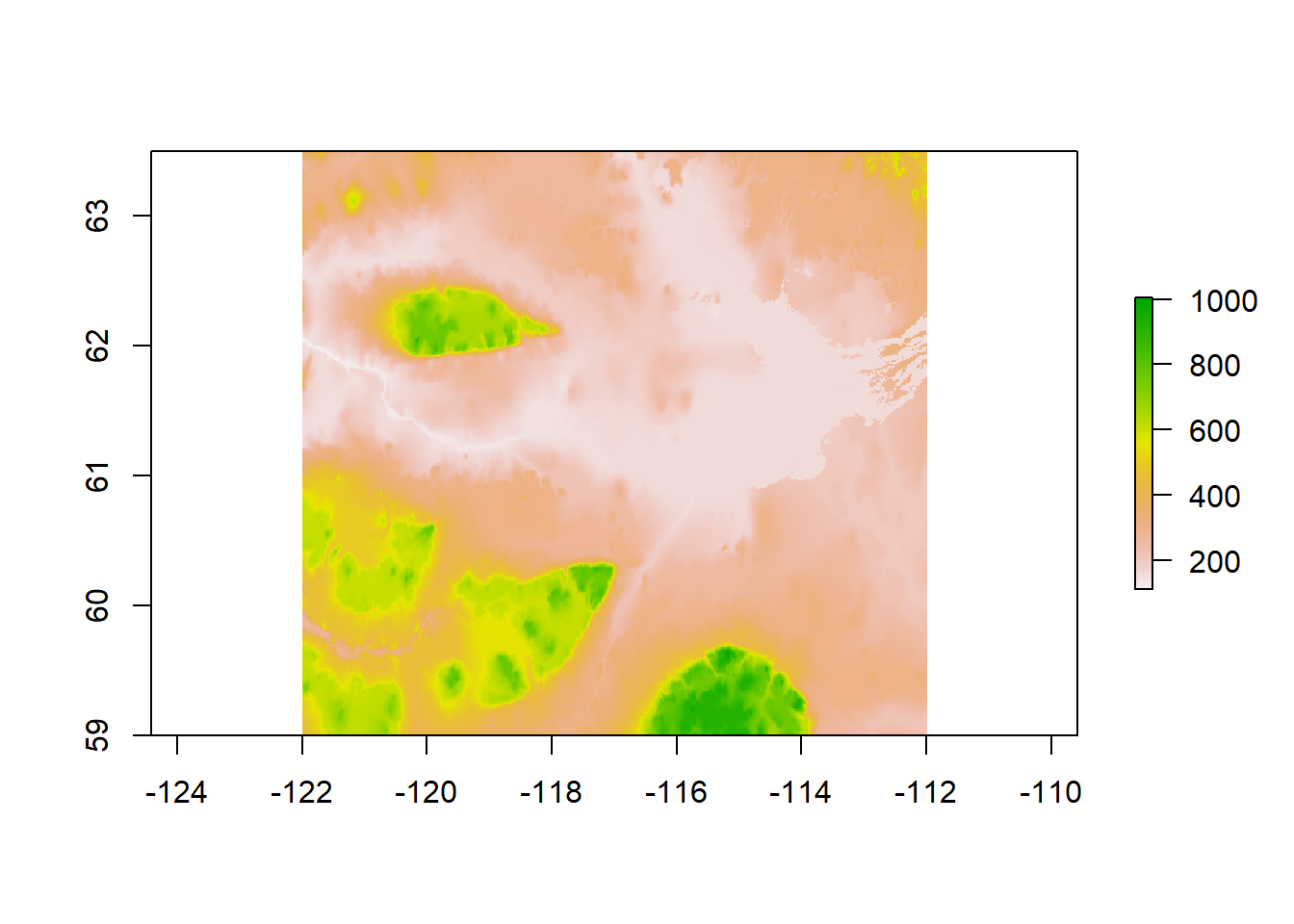
A very nice, clear image of Great Slave Lake, the Mackenzie river that drains it and several elevated plateaus. These data are in lat-long. We can compare the projections of the our other objects:
projection(elevation)## [1] "+proj=longlat +datum=WGS84 +no_defs +ellps=WGS84 +towgs84=0,0,0"projection(wbnp)## [1] "+proj=longlat +datum=WGS84 +no_defs +ellps=WGS84 +towgs84=0,0,0"projection(lines2010)## [1] "+proj=lcc +lat_1=50 +lat_2=70 +lat_0=40 +lon_0=-96 +x_0=0 +y_0=0 +datum=NAD83 +units=m +no_defs +ellps=GRS80 +towgs84=0,0,0"One of these does not belong! But we can easily reproject, and visualize everything at once:
lines2010.ll <- spTransform(lines2010, projection(elevation))
plot(elevation, col = grey.colors(100, start = 0))
plot(wbnp, col = alpha("green", 0.3), add = TRUE, bor = NA)
plot(lines2010.ll, add = TRUE, col = c("blue", "brown", "red", "green", "white",
    "pink", "white")[lines2010.utm$Class], lty = legend.args$lty[lines2010.utm$Class],
    lwd = legend.args$lwd[lines2010.utm$Class])
with(caribou[seq(1, nrow(caribou), 100), ], points(Longitude, Latitude, col = alpha(as.integer(Herd),
    0.2), pch = 19, cex = 0.5))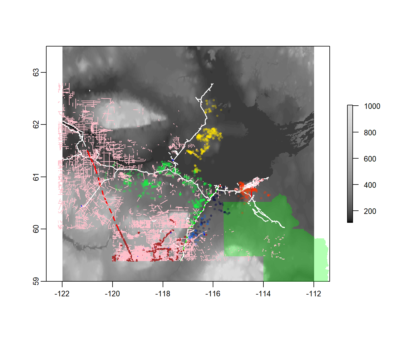
3.2 Discrete: Land classes
A discrete raster is found in the landcover.tif file. This one is the International Geosphere–Biosphere Programme (IGBP) land classification, downloaded for North America from the Global Land Cover Classification (GLCC) product at Earth Explorer.
landcover <- raster("./_data/landcover.tif")
landcover
## class : RasterLayer
## dimensions : 480, 482, 231360 (nrow, ncol, ncell)
## resolution : 1000, 1000 (x, y)
## extent : -1211500, -729500, 1114500, 1594500 (xmin, xmax, ymin, ymax)
## coord. ref. : +proj=laea +lat_0=50 +lon_0=-100 +x_0=0 +y_0=0 +a=6370997 +b=6370997 +units=m +no_defs
## data source : C:\Users\elie\Box Sync\teaching\NWT2018\materials\_data\landcover.tif
## names : landcover
## values : 1, 17 (min, max)plot(landcover)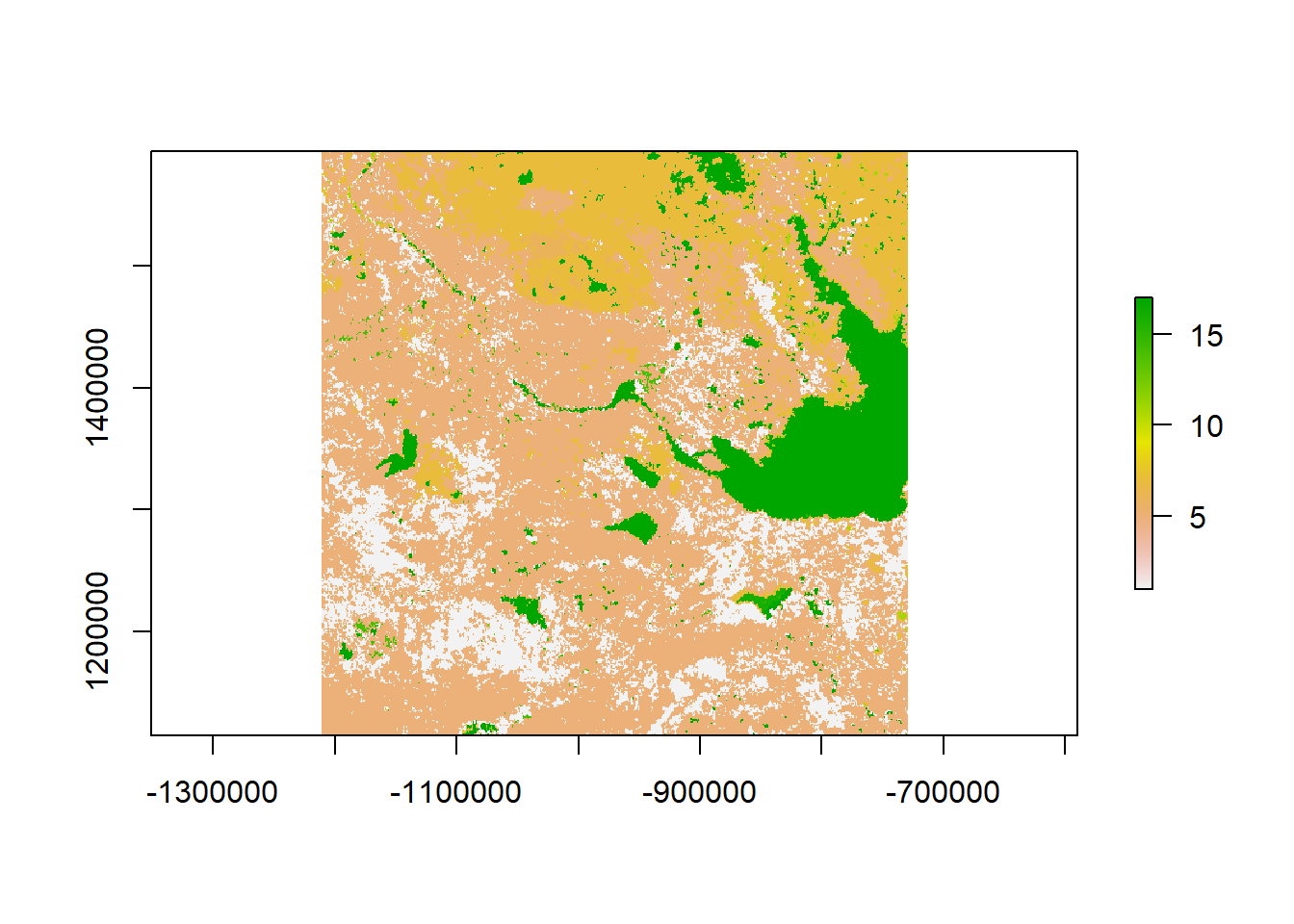
It’s unclear from this image what the colors or numbers mean. But here is the list of values:
values(landcover)[1:100]## [1] 5 6 5 5 5 5 1 5 5 5 5 5 5 5 5 5 1 5 5 5 7 7 7
## [24] 5 5 1 5 5 5 5 5 5 5 5 5 5 5 5 5 5 1 11 11 7 5 7
## [47] 7 1 5 5 5 5 5 5 5 5 5 5 5 5 5 5 5 5 5 7 7 7 7
## [70] 7 7 7 7 5 5 7 5 5 5 7 7 7 7 5 7 7 7 7 7 7 7 5
## [93] 5 7 7 7 7 7 6 6The run-down of the IGBP land classes is here: https://lta.cr.usgs.gov/glcc/nadoc2_0#igbp. Unfortunately, this particular raster doesn’t contain the interpretations of the value (many do).
I downloaded this table and added some colors that I thought would help.
landcover.legend <- read.csv("./_data/landcover.legend.csv")
landcover.legend$Color <- as.character(landcover.legend$Color)| Value | Type | Color |
|---|---|---|
| 1 | Evergreen Needleleaf Forest | darkgreen |
| 2 | Evergreen Broadleaf Forest | NA |
| 3 | Deciduous Needleleaf Forest | NA |
| 4 | Deciduous Broadleaf Forest | NA |
| 5 | Mixed Forest | green |
| 6 | Closed Shrublands | yellowgreen |
| 7 | Open Shrublands | antiquewhite |
| 8 | Woody Savannas | NA |
| 9 | Savannas | NA |
| 10 | Grasslands | lightgreen |
| 11 | Permanent Wetlands | brown |
| 12 | Croplands | yellow |
| 13 | Urban and Built-Up | grey |
| 14 | Cropland/Natural Vegetation Mosaic | pink |
| 15 | Snow and Ice | lightblue |
| 16 | Barren or Sparsely Vegetated | indianred2 |
| 17 | Water Bodies | navy |
Here’s a plot with the colorcoded and labeled landclasses:
image(landcover, col = landcover.legend$Color, asp = 1)
with(na.omit(landcover.legend), legend("bottomleft", fill = Color, legend = Type,
    cex = 0.6, ncol = 2, bg = "white"))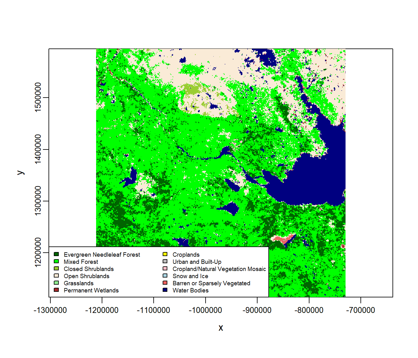
3.3 Projecting rasters
As usual, we need to retransform to have all of our data in the same coordinate system. This raster is in something called “laea” - another Lambert, I guess:
projection(landcover)## [1] "+proj=laea +lat_0=50 +lon_0=-100 +x_0=0 +y_0=0 +a=6370997 +b=6370997 +units=m +no_defs"We’ll like to project the raster into the UTM of our other covariates - and make sure that everything matches. For rasters, this is not quite as simple as for spatial polygons, because the raster is necessarily composed of rectangular grids! We’re going to have to (a) recreate a NEW raster with the properties we want, (b) populate it with values from the old raster with projectRaster command. Note that we’ll have to do this both for the elevation and the landcover
landcover.utm <- raster(nrows = 180, ncols = 180, ext = extent(lines2010.utm),
    crs = projection(lines2010.utm))
elevation.utm <- landcover.utm

landcover.utm <- projectRaster(from = landcover, to = landcover.utm, method = "ngb")
elevation.utm <- projectRaster(from = elevation, to = elevation.utm, method = "ngb")

plot(landcover.utm, col = landcover.legend$Color)
with(caribou[seq(1, nrow(caribou), 100), ], points(X, Y, pch = 19, col = "red",
    cex = 0.5))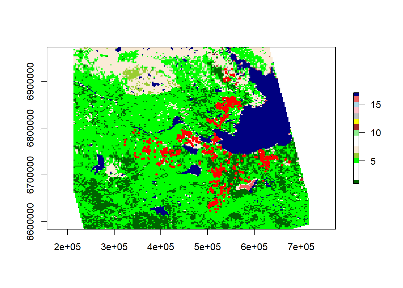
3.4 Making a RasterBrick
Sometimes it can be handy to have a RasterBrick - which is a bunch of rasters (of the same “extent”) stacked on top of each other. Since elevation and landcover now have the same extent and projection, this is easy to do:
r <- brick(landcover.utm, nl = 2)
r[[2]] <- elevation.utm
plot(r)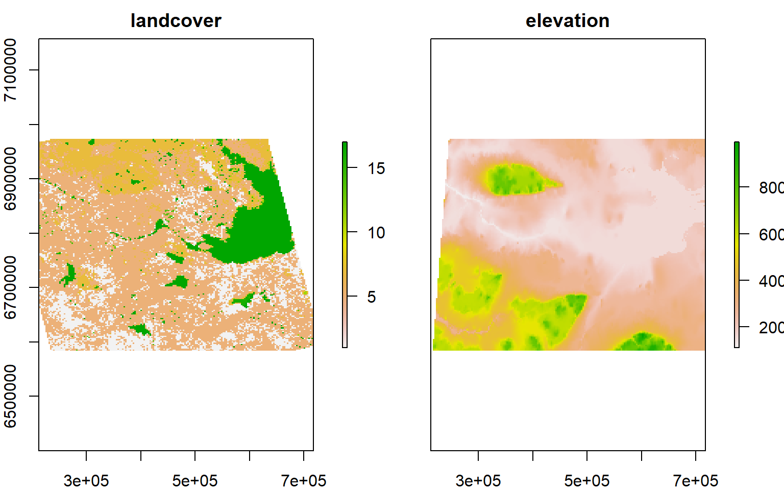
4 Saving all the spatial data
For efficiency (and to save the need to replicate a lot of code), you can save all of the correctly transformed habitat covariates in a single file which will be easy to open as needed.
landcover <- landcover.utm
elevation <- elevation.utm
lines2010 <- lines2010.utm
save(lines2010, elevation, landcover, landcover.legend, file = "./_data/habitatdata.rda")