Lab: Bayesian Lilacs - an MCMC
BIOL709/BSCI339
R Markdown
First …. packages!
packages <- c("ggplot2", "ggmap", "plyr", "magrittr", "rstan", "coda", "lattice")
sapply(packages, require, char = TRUE)
## ggplot2 ggmap plyr magrittr rstan coda lattice
## TRUE TRUE TRUE TRUE TRUE TRUE TRUE1. Lilac Data
Beautiful lilac flowering data are here: ftp://ftp.ncdc.noaa.gov/pub/data/paleo/phenology/north_america_lilac.txt
I tidied the data and posted them to the website here:
ll <- read.csv("https://terpconnect.umd.edu/~egurarie/teaching/Biol709/data/LilacLocations.csv")
lp <- read.csv("https://terpconnect.umd.edu/~egurarie/teaching/Biol709/data/LilacPhenology.csv")
The lilac locations have latitudes, longitudes and eleveations:
head(ll)## X ID STATION State Lat Long Elev Nobs
## 1 1 20309 APACHE POWDER COMPANY AZ 31.54 -110.16 1125.00 9
## 2 2 20958 BOWIE AZ 32.20 -109.29 1145.12 6
## 3 3 21101 BURRUS RANCH AZ 35.16 -111.32 2073.17 9
## 4 4 21614 CHILDS AZ 34.21 -111.42 807.93 6
## 5 5 21634 CHINLE AZ 36.09 -109.32 1688.41 10
## 6 6 21749 CIBECUE AZ 34.03 -110.27 1615.85 8The lilac phenology contains, importantly, the day of blooming (our response variable) across years at each station.
head(lp)## STATION YEAR SPECIES LEAF BLOOM
## 1 20309 1957 2 NA 67
## 2 20309 1958 2 NA 90
## 3 20309 1959 2 NA 92
## 4 20309 1960 2 NA 79
## 5 20309 1961 2 NA 78
## 6 20309 1962 2 NA 88Map all these data with ggmap():
require(ggmap)
basemap1 <- get_map(location = c(-112, 38), maptype = "terrain", zoom=4)
ggmap(basemap1) + geom_point(data = ll, mapping = aes(x = Long, y = Lat, colour = Elev, size = Nobs))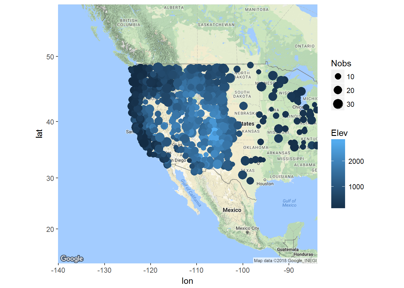
Pick out a few widely scattered stations (try this and all of the following with your own set!)
Stations <- c(456624, 426357, 354147, 456974)
subset(ll, ID %in% Stations)
## X ID STATION State Lat Long Elev Nobs
## 779 779 354147 IMNAHA OR 45.34 -116.50 564.02 30
## 894 894 426357 OAK CITY UT 39.23 -112.20 1547.26 32
## 986 986 456624 PORT ANGELES WA 48.07 -123.26 60.98 28
## 994 994 456974 REPUBLIC WA 48.39 -118.44 792.68 35and tidy the data:
lilacs <- subset(lp, STATION %in% Stations)
lilacs <- lilacs[!is.na(lilacs$BLOOM),]
Plot some trends over time, with a “smoother” in ggplot:
require(ggplot2)
ggplot(lilacs, aes(x=YEAR, y=BLOOM)) +
  geom_point() +
  facet_grid(.~STATION) +
  stat_smooth()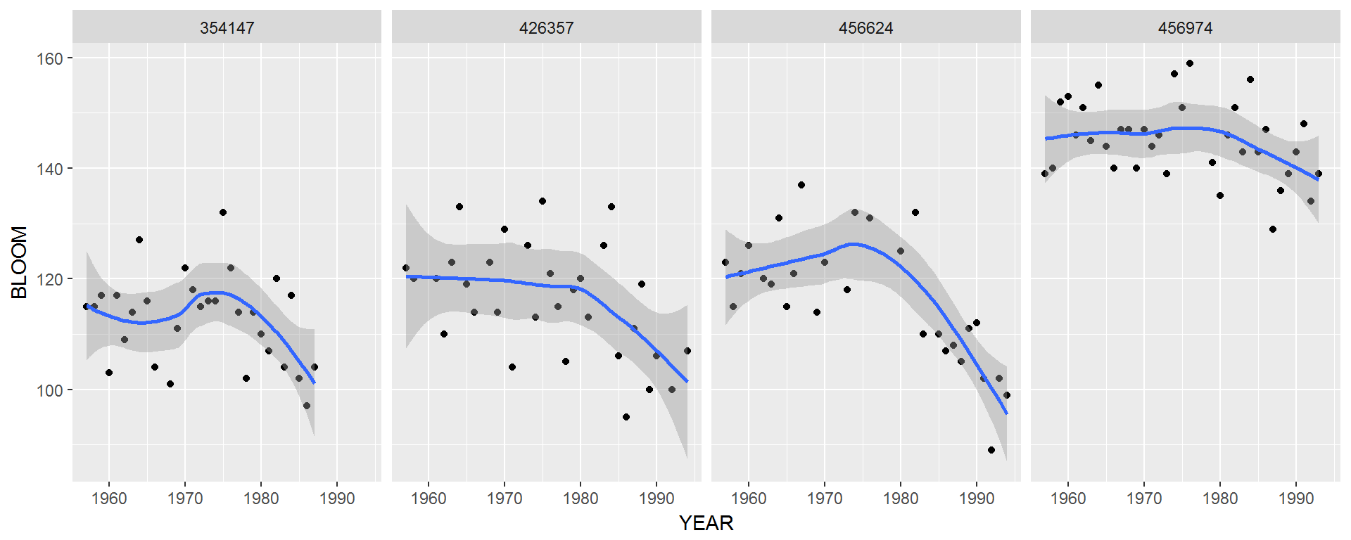
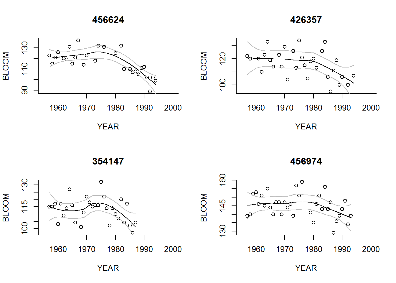
Note: It is easy and seductive to make figures like the above - but an imnportant problem with any black box method (like stat_smooth()) is that the actual tool is obscured. In this case, the smoother is “loess” (localized regression). Replicating the figure in base plot is a good way to control that you
for(s in Stations)
{
  years <- 1955:2000
  mydata <- subset(lilacs, STATION==s)
  with(mydata, plot(YEAR, BLOOM, main=s, xlim=range(years)))
  myloess <- loess(BLOOM~YEAR, data=mydata)
  myloess.predict <- predict(myloess, data.frame(YEAR = years), se=TRUE)
  with(myloess.predict, lines(years, fit))
  with(myloess.predict, lines(years, fit))
  with(myloess.predict, lines(years, fit - 2*se.fit, col="grey"))
  with(myloess.predict, lines(years, fit + 2*se.fit, col="grey"))
}
Here are our selected stations:
basemap2 <- get_map(location = c(-120, 45), maptype = "terrain", zoom=5)
ggmap(basemap2) +
  geom_point(data = subset(ll, ID %in% Stations), aes(x = Long, y = Lat, colour = Elev), size = 5) +
geom_text(data = subset(ll, ID %in% Stations), aes(x = Long, y = Lat+1), color = "red", label=Stations) 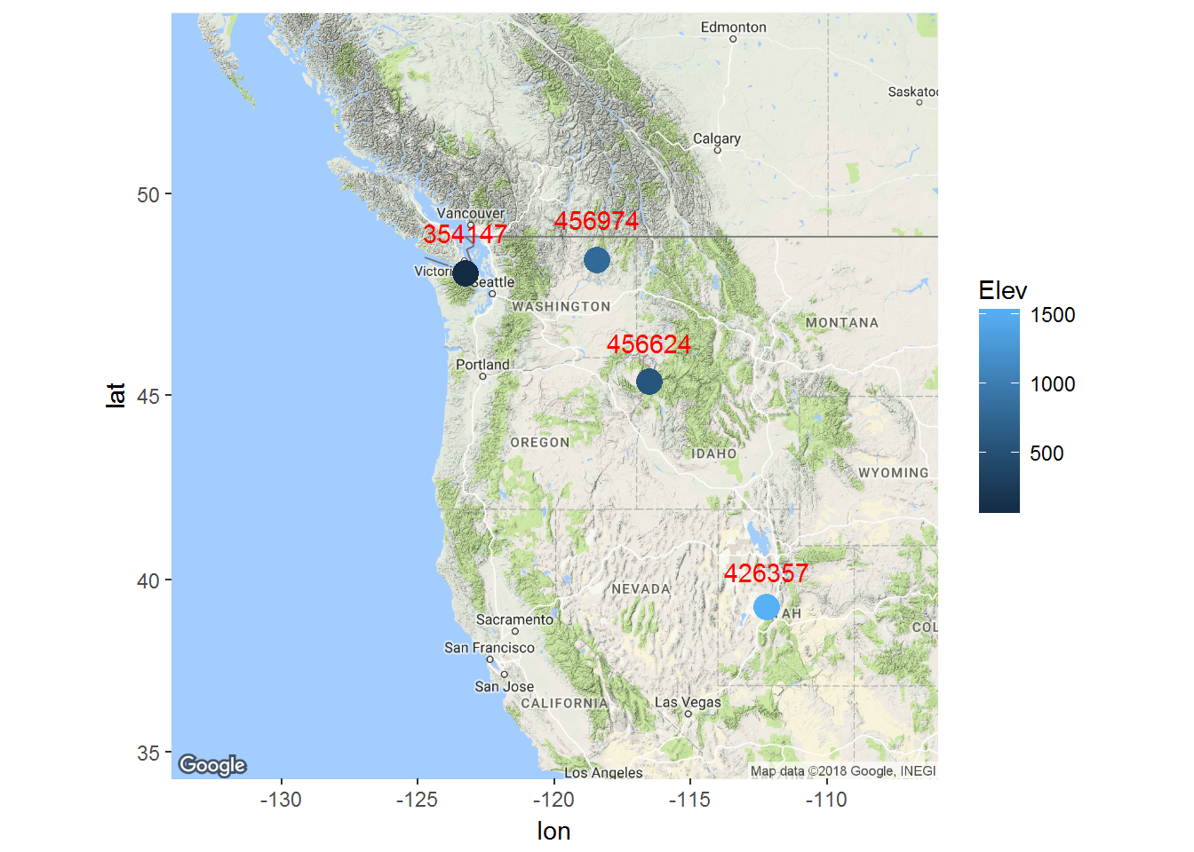
2. A model for blooming time
It looks like the blooming time of lilacs since 1980 has started happening earlier and earlier. We propose a hockeystick model, i.e.: \[ X_{i,j}(T) = \begin{cases} \beta_0 + \epsilon_{ij} & T < \tau \\ \beta_0 + \beta_1(T - \tau) + \epsilon_{ij} & T \geq \tau \end{cases} \]
Encode the model in R (note the ifelse() function):
getX.hat <- function(T, beta0, beta1, tau)
  ifelse(T < tau, beta0, beta0 + beta1 * (T-tau))
Guess some values, and see how it looks. We’ll focus on just one station, and make things easier by extracting htose columns:
l1 <- subset(lilacs, STATION == Stations[1])
p <- c(120, -2, 1980, 1)
plot(BLOOM~YEAR, pch = 19, col="grey", data = l1)
lines(l1$YEAR, getX.hat(l1$YEAR, beta0=120, beta1 = -2, tau = 1980), col=2, lwd=2)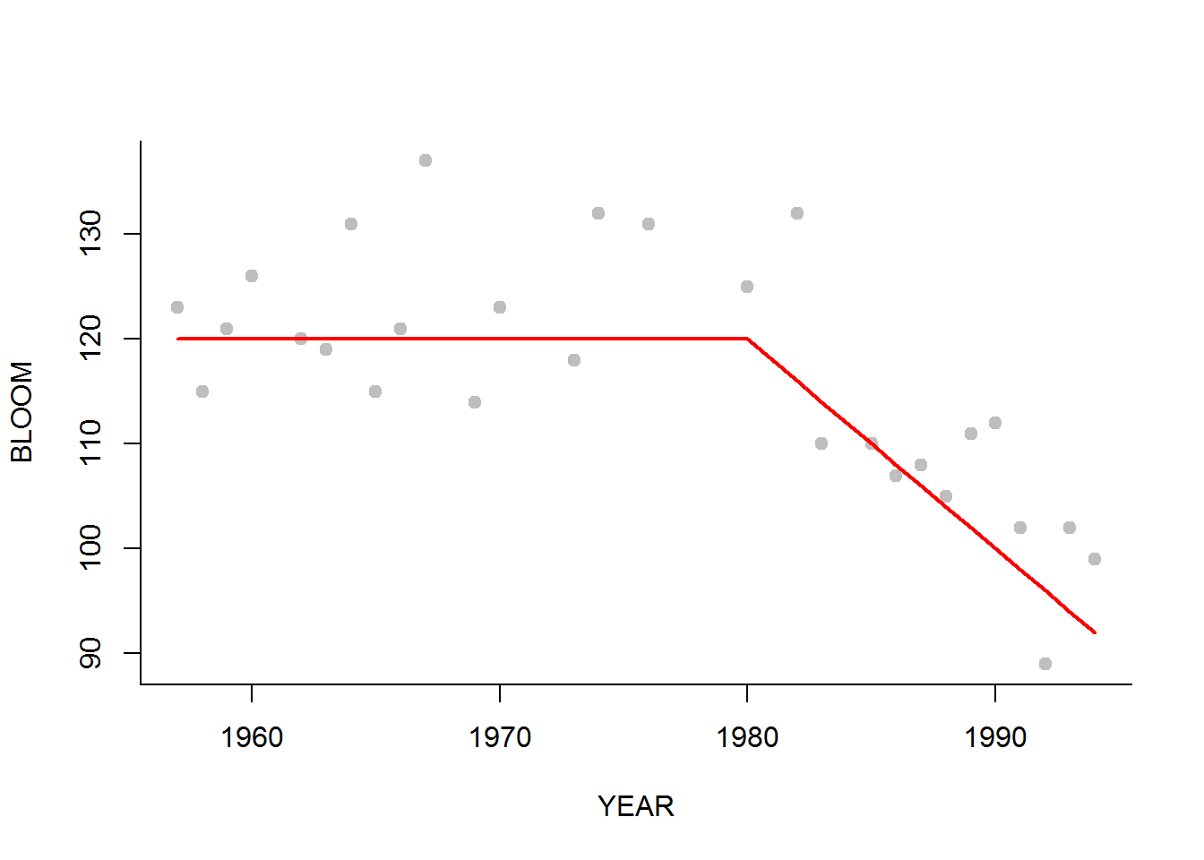
Ok, before we run off to analyze this model, lets first encode a simple linear regression in STAN:
3. Simple STAN example: a linear model
The basic idea of using RSTAN is:
- Encode model in STAN-specific code
- Use Rstan (which uses Rcpp) to compile the MCMC sampler as an R-accessible piece of C++ code
- Run the sampler - specifying the data, the number of iterations, chains, etc.
- Analyze the resulting chains for convergence and stationarity.
Step I. Writing the code.
STAN uses a pseudo-R pseudo-C type. The specifications and examples are given in the very useful manual here: http://mc-stan.org/manual.html
Here is an example of the linear model, coded in STAN:
data {
  int<lower=0> n; //
  vector[n] y; // Y Vector
  vector[n] x; // X Vector
}

parameters {
  real beta0;                   // intercept
  real beta1;                   // slope
  real<lower=0> sigma;  // standard deviation
}

model {
  //Declare variable
  vector[n] yhat;

  //Priors
  sigma ~ inv_gamma(0.001, 0.001);
  beta0 ~ normal(150,150);
  beta1 ~ normal(0, 10);

  //model
  for(i in 1:n){
   yhat[i] = beta0 + beta1 * (x[i] - mean(x));}
  y ~ normal(yhat, sigma);
}
There are several pieces (called “blocks”) here to go over.
- data block: This informs Stan of the objects that we will be passing to it (as a list, from within R). In this case we have 1 constants and a few vectors. Note, you need to specify
nbecause it is used later in the model specification. - parameters block: where you specify the parameters to estimate. Note, the types are important, and that you can set lower and upper limits to them easily.
- model block: is the meat of the model Note that the
yhatvariable is one more vector that must be defined - and all variables must be specified at the beginning of the block. Note, also, I put in a loop to define theyhat, to illustrate the loop syntax. But in fact STAN is quite good at vectorization, and that vectorization can be somewhat and that loop could be replaced simply with:
yhat <- beta0 + beta1 * (x - mean(x));In principle STAN code is straightforward, but there are always traps and pitfalls, that take a while to debug (and involve a fair amount of looking at the manual and googling errors).
Note that the priors I selected were fairly uninformative. The inverse gamma distribution with low values of \(\alpha\) and \(\beta\) is a common one for the variance, which should be positive.
Step II. Compiling
The big step (the SLOW step) is the transformation of the STAN specification to C++ code, and then compilation of that code. This is done with the command stan_model. In theory you could do this in-line, but the best way is to save the STAN code (e.g., save the STAN code above as lm.stan in your working directory) and call it from the command line as follows.
require(rstan)
lm_stan <- stan_model(file = "lm.stan")
This takes a few minutes to perform on my computer. Compiled versions (of all the Stan models in this lab) can be found here:http://faculty.washington.edu/eliezg/teaching/StatR503/stanmodels/
Step III. Running the MCMC
To actually run the MCMC on the data and the model you use the sampling command. A few things to note:
- the
Datamust be a named list with the variable names and types corresponding strictly to the definition sin thedatablock of the stan model.
- There are lots of detailed options with respect to the sampling, but the default is: 4 chains, each of length 2000, of which the first 1000 are trimmed (“warmup”).
Data <- with(l1, list(n = nrow(l1), x = YEAR, y = BLOOM))
lm.fit <- sampling(lm_stan, Data)
##
## SAMPLING FOR MODEL 'lm' NOW (CHAIN 1).
##
## Gradient evaluation took 0 seconds
## 1000 transitions using 10 leapfrog steps per transition would take 0 seconds.
## Adjust your expectations accordingly!
##
##
## Iteration: 1 / 2000 [ 0%] (Warmup)
## Iteration: 200 / 2000 [ 10%] (Warmup)
## Iteration: 400 / 2000 [ 20%] (Warmup)
## Iteration: 600 / 2000 [ 30%] (Warmup)
## Iteration: 800 / 2000 [ 40%] (Warmup)
## Iteration: 1000 / 2000 [ 50%] (Warmup)
## Iteration: 1001 / 2000 [ 50%] (Sampling)
## Iteration: 1200 / 2000 [ 60%] (Sampling)
## Iteration: 1400 / 2000 [ 70%] (Sampling)
## Iteration: 1600 / 2000 [ 80%] (Sampling)
## Iteration: 1800 / 2000 [ 90%] (Sampling)
## Iteration: 2000 / 2000 [100%] (Sampling)
##
## Elapsed Time: 0.027 seconds (Warm-up)
## 0.021 seconds (Sampling)
## 0.048 seconds (Total)
##
##
## SAMPLING FOR MODEL 'lm' NOW (CHAIN 2).
##
## Gradient evaluation took 0 seconds
## 1000 transitions using 10 leapfrog steps per transition would take 0 seconds.
## Adjust your expectations accordingly!
##
##
## Iteration: 1 / 2000 [ 0%] (Warmup)
## Iteration: 200 / 2000 [ 10%] (Warmup)
## Iteration: 400 / 2000 [ 20%] (Warmup)
## Iteration: 600 / 2000 [ 30%] (Warmup)
## Iteration: 800 / 2000 [ 40%] (Warmup)
## Iteration: 1000 / 2000 [ 50%] (Warmup)
## Iteration: 1001 / 2000 [ 50%] (Sampling)
## Iteration: 1200 / 2000 [ 60%] (Sampling)
## Iteration: 1400 / 2000 [ 70%] (Sampling)
## Iteration: 1600 / 2000 [ 80%] (Sampling)
## Iteration: 1800 / 2000 [ 90%] (Sampling)
## Iteration: 2000 / 2000 [100%] (Sampling)
##
## Elapsed Time: 0.03 seconds (Warm-up)
## 0.038 seconds (Sampling)
## 0.068 seconds (Total)
##
##
## SAMPLING FOR MODEL 'lm' NOW (CHAIN 3).
##
## Gradient evaluation took 0 seconds
## 1000 transitions using 10 leapfrog steps per transition would take 0 seconds.
## Adjust your expectations accordingly!
##
##
## Iteration: 1 / 2000 [ 0%] (Warmup)
## Iteration: 200 / 2000 [ 10%] (Warmup)
## Iteration: 400 / 2000 [ 20%] (Warmup)
## Iteration: 600 / 2000 [ 30%] (Warmup)
## Iteration: 800 / 2000 [ 40%] (Warmup)
## Iteration: 1000 / 2000 [ 50%] (Warmup)
## Iteration: 1001 / 2000 [ 50%] (Sampling)
## Iteration: 1200 / 2000 [ 60%] (Sampling)
## Iteration: 1400 / 2000 [ 70%] (Sampling)
## Iteration: 1600 / 2000 [ 80%] (Sampling)
## Iteration: 1800 / 2000 [ 90%] (Sampling)
## Iteration: 2000 / 2000 [100%] (Sampling)
##
## Elapsed Time: 0.027 seconds (Warm-up)
## 0.021 seconds (Sampling)
## 0.048 seconds (Total)
##
##
## SAMPLING FOR MODEL 'lm' NOW (CHAIN 4).
##
## Gradient evaluation took 0 seconds
## 1000 transitions using 10 leapfrog steps per transition would take 0 seconds.
## Adjust your expectations accordingly!
##
##
## Iteration: 1 / 2000 [ 0%] (Warmup)
## Iteration: 200 / 2000 [ 10%] (Warmup)
## Iteration: 400 / 2000 [ 20%] (Warmup)
## Iteration: 600 / 2000 [ 30%] (Warmup)
## Iteration: 800 / 2000 [ 40%] (Warmup)
## Iteration: 1000 / 2000 [ 50%] (Warmup)
## Iteration: 1001 / 2000 [ 50%] (Sampling)
## Iteration: 1200 / 2000 [ 60%] (Sampling)
## Iteration: 1400 / 2000 [ 70%] (Sampling)
## Iteration: 1600 / 2000 [ 80%] (Sampling)
## Iteration: 1800 / 2000 [ 90%] (Sampling)
## Iteration: 2000 / 2000 [100%] (Sampling)
##
## Elapsed Time: 0.027 seconds (Warm-up)
## 0.023 seconds (Sampling)
## 0.05 seconds (Total)A brief summary of the results:
lm.fit## Inference for Stan model: lm.
## 4 chains, each with iter=2000; warmup=1000; thin=1;
## post-warmup draws per chain=1000, total post-warmup draws=4000.
##
## mean se_mean sd 2.5% 25% 50% 75% 97.5% n_eff Rhat
## beta0 116.38 0.03 1.79 112.71 115.24 116.39 117.57 119.91 3467 1.00
## beta1 -0.60 0.00 0.14 -0.89 -0.69 -0.60 -0.51 -0.31 2751 1.00
## sigma 9.14 0.02 1.28 7.08 8.20 9.00 9.91 11.97 2925 1.00
## lp__ -75.61 0.04 1.32 -79.06 -76.16 -75.28 -74.66 -74.14 1317 1.01
##
## Samples were drawn using NUTS(diag_e) at Fri Jan 19 13:33:39 2018.
## For each parameter, n_eff is a crude measure of effective sample size,
## and Rhat is the potential scale reduction factor on split chains (at
## convergence, Rhat=1).This takes under a second to perform on my machine.
You can see from the output that the regression coefficients are around 116.5 and 0,6, with a standard deviation of 9.3. It is easy (of course) to compare these results with a straightforward OLS:
summary(lm(BLOOM ~ I(YEAR-mean(YEAR)), data = l1))##
## Call:
## lm(formula = BLOOM ~ I(YEAR - mean(YEAR)), data = l1)
##
## Residuals:
## Min 1Q Median 3Q Max
## -17.565 -5.131 -1.802 3.396 19.382
##
## Coefficients:
## Estimate Std. Error t value Pr(>|t|)
## (Intercept) 116.3571 1.6717 69.606 < 2e-16 ***
## I(YEAR - mean(YEAR)) -0.6052 0.1374 -4.405 0.000162 ***
## ---
## Signif. codes: 0 '***' 0.001 '**' 0.01 '*' 0.05 '.' 0.1 ' ' 1
##
## Residual standard error: 8.846 on 26 degrees of freedom
## Multiple R-squared: 0.4273, Adjusted R-squared: 0.4053
## F-statistic: 19.4 on 1 and 26 DF, p-value: 0.0001617The estimate of standard deviation is given by:
summary(lm(BLOOM ~ I(YEAR-mean(YEAR)), data = l1))$sigma## [1] 8.845546Should be a pretty good match.
Step IV. Diagnosing the MCMC
To apply the coda family of diagnostic tools, you need to extract the chains from the STAN fitted object, and re-create it is as an mcmc.list. This is done with the As.mcmc.list command.
require(coda)
lm.chains <- As.mcmc.list(lm.fit, pars =  c("beta0", "beta1", "sigma"))
plot(lm.chains)
You can see that the chains seem fairly well behaved, i.e. they converge and the densities are consistent between chains. Here is a nicer looking plot of the posterior distributions:
require(lattice)
densityplot(lm.chains)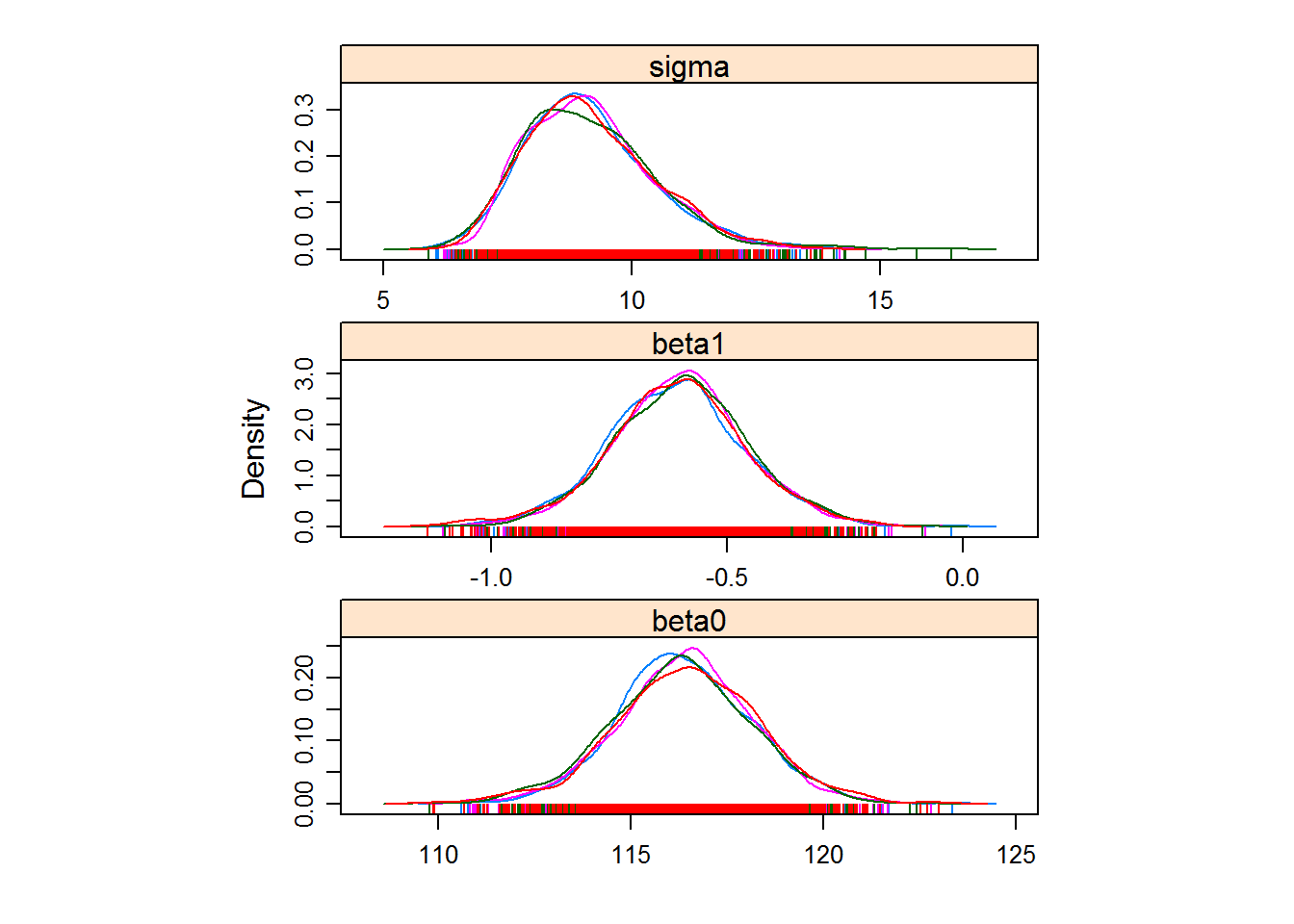
4. Hockeystick model
Ok, now we will try to fit this hockeystick model to one of these datasets. Note that the version below basically adjusts the lm.stan model with just a few tweaks, adding that important step function via the STAN function int_step (which is 0 when the argument is less than 0, and 1 when the argument is greater than 0):
data {
  int<lower=0> n; //
  vector[n] y; // Y Vector
  vector[n] x; // X Vector
}

parameters {
  real beta0;  // intercept
  real beta1;  // slope
  real<lower=min(x), upper=max(x)> tau;    // changepoint
  real<lower=0> sigma;   // variance
}

model {
    vector[n] yhat;

  // Priors
    sigma ~ inv_gamma(0.001, 0.001);
    beta0 ~ normal(150,150);
    beta1 ~ normal(0, 10);
    tau ~ uniform(min(x), max(x));
  // Define the mean
  for(i in 1:n)
    yhat[i] = beta0 + int_step(x[i]-tau)*beta1*(x[i] - tau);

  // likelihood / probability model
    y ~ normal(yhat, sigma);
}
Compile:
hockeystick_stan <- stan_model(file = "./_stanmodels/hockeystick.stan")hockeystick.fit <- sampling(hockeystick_stan, Data)##
## SAMPLING FOR MODEL 'hockeystick' NOW (CHAIN 1).
##
## Gradient evaluation took 0 seconds
## 1000 transitions using 10 leapfrog steps per transition would take 0 seconds.
## Adjust your expectations accordingly!
##
##
## Iteration: 1 / 2000 [ 0%] (Warmup)
## Iteration: 200 / 2000 [ 10%] (Warmup)
## Iteration: 400 / 2000 [ 20%] (Warmup)
## Iteration: 600 / 2000 [ 30%] (Warmup)
## Iteration: 800 / 2000 [ 40%] (Warmup)
## Iteration: 1000 / 2000 [ 50%] (Warmup)
## Iteration: 1001 / 2000 [ 50%] (Sampling)
## Iteration: 1200 / 2000 [ 60%] (Sampling)
## Iteration: 1400 / 2000 [ 70%] (Sampling)
## Iteration: 1600 / 2000 [ 80%] (Sampling)
## Iteration: 1800 / 2000 [ 90%] (Sampling)
## Iteration: 2000 / 2000 [100%] (Sampling)
##
## Elapsed Time: 0.059 seconds (Warm-up)
## 0.052 seconds (Sampling)
## 0.111 seconds (Total)
##
##
## SAMPLING FOR MODEL 'hockeystick' NOW (CHAIN 2).
##
## Gradient evaluation took 0 seconds
## 1000 transitions using 10 leapfrog steps per transition would take 0 seconds.
## Adjust your expectations accordingly!
##
##
## Iteration: 1 / 2000 [ 0%] (Warmup)
## Iteration: 200 / 2000 [ 10%] (Warmup)
## Iteration: 400 / 2000 [ 20%] (Warmup)
## Iteration: 600 / 2000 [ 30%] (Warmup)
## Iteration: 800 / 2000 [ 40%] (Warmup)
## Iteration: 1000 / 2000 [ 50%] (Warmup)
## Iteration: 1001 / 2000 [ 50%] (Sampling)
## Iteration: 1200 / 2000 [ 60%] (Sampling)
## Iteration: 1400 / 2000 [ 70%] (Sampling)
## Iteration: 1600 / 2000 [ 80%] (Sampling)
## Iteration: 1800 / 2000 [ 90%] (Sampling)
## Iteration: 2000 / 2000 [100%] (Sampling)
##
## Elapsed Time: 0.062 seconds (Warm-up)
## 0.053 seconds (Sampling)
## 0.115 seconds (Total)
##
##
## SAMPLING FOR MODEL 'hockeystick' NOW (CHAIN 3).
##
## Gradient evaluation took 0 seconds
## 1000 transitions using 10 leapfrog steps per transition would take 0 seconds.
## Adjust your expectations accordingly!
##
##
## Iteration: 1 / 2000 [ 0%] (Warmup)
## Iteration: 200 / 2000 [ 10%] (Warmup)
## Iteration: 400 / 2000 [ 20%] (Warmup)
## Iteration: 600 / 2000 [ 30%] (Warmup)
## Iteration: 800 / 2000 [ 40%] (Warmup)
## Iteration: 1000 / 2000 [ 50%] (Warmup)
## Iteration: 1001 / 2000 [ 50%] (Sampling)
## Iteration: 1200 / 2000 [ 60%] (Sampling)
## Iteration: 1400 / 2000 [ 70%] (Sampling)
## Iteration: 1600 / 2000 [ 80%] (Sampling)
## Iteration: 1800 / 2000 [ 90%] (Sampling)
## Iteration: 2000 / 2000 [100%] (Sampling)
##
## Elapsed Time: 0.059 seconds (Warm-up)
## 0.054 seconds (Sampling)
## 0.113 seconds (Total)
##
##
## SAMPLING FOR MODEL 'hockeystick' NOW (CHAIN 4).
##
## Gradient evaluation took 0 seconds
## 1000 transitions using 10 leapfrog steps per transition would take 0 seconds.
## Adjust your expectations accordingly!
##
##
## Iteration: 1 / 2000 [ 0%] (Warmup)
## Iteration: 200 / 2000 [ 10%] (Warmup)
## Iteration: 400 / 2000 [ 20%] (Warmup)
## Iteration: 600 / 2000 [ 30%] (Warmup)
## Iteration: 800 / 2000 [ 40%] (Warmup)
## Iteration: 1000 / 2000 [ 50%] (Warmup)
## Iteration: 1001 / 2000 [ 50%] (Sampling)
## Iteration: 1200 / 2000 [ 60%] (Sampling)
## Iteration: 1400 / 2000 [ 70%] (Sampling)
## Iteration: 1600 / 2000 [ 80%] (Sampling)
## Iteration: 1800 / 2000 [ 90%] (Sampling)
## Iteration: 2000 / 2000 [100%] (Sampling)
##
## Elapsed Time: 0.062 seconds (Warm-up)
## 0.058 seconds (Sampling)
## 0.12 seconds (Total)This takes a little bit longer to fit, but still just on the order of seconds.
Look at the estimates:
hockeystick.fit## Inference for Stan model: hockeystick.
## 4 chains, each with iter=2000; warmup=1000; thin=1;
## post-warmup draws per chain=1000, total post-warmup draws=4000.
##
## mean se_mean sd 2.5% 25% 50% 75% 97.5% n_eff
## beta0 123.19 0.04 1.78 119.74 122.00 123.21 124.34 126.71 2323
## beta1 -1.94 0.01 0.50 -2.96 -2.25 -1.91 -1.58 -1.06 1853
## tau 1979.72 0.06 2.65 1973.74 1978.37 1980.12 1981.44 1983.96 1683
## sigma 7.13 0.02 1.08 5.42 6.36 6.97 7.76 9.58 1882
## lp__ -66.47 0.05 1.62 -70.61 -67.24 -66.06 -65.28 -64.55 1077
## Rhat
## beta0 1
## beta1 1
## tau 1
## sigma 1
## lp__ 1
##
## Samples were drawn using NUTS(diag_e) at Fri Jan 19 13:33:42 2018.
## For each parameter, n_eff is a crude measure of effective sample size,
## and Rhat is the potential scale reduction factor on split chains (at
## convergence, Rhat=1).They look quite reasonable and converged!
Let’s assess the fits:
require(lattice)
hockeystick.mcmc <- As.mcmc.list(hockeystick.fit, c("beta0", "beta1","tau","sigma"))
xyplot(hockeystick.mcmc)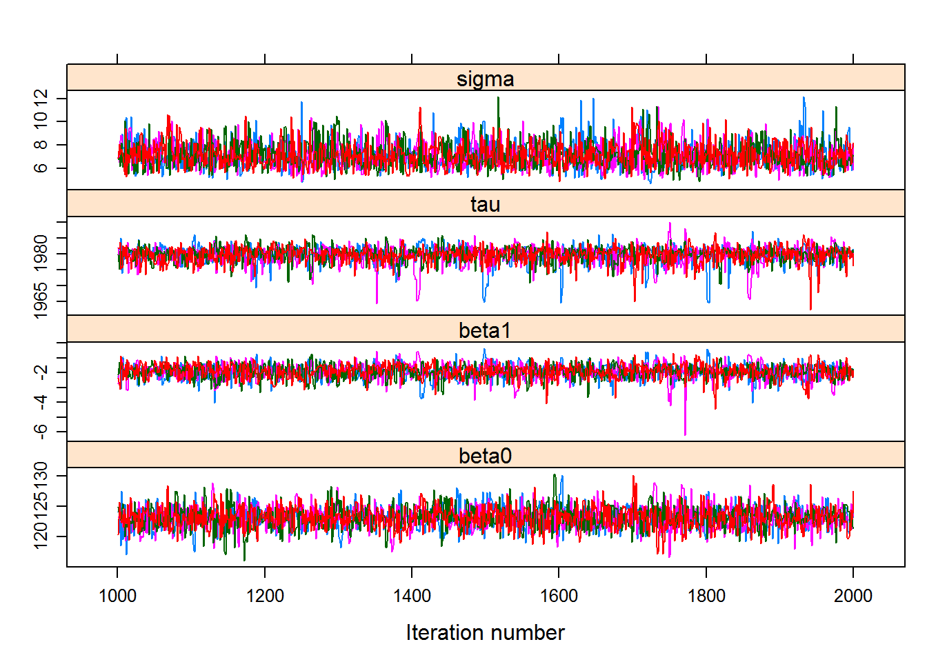
densityplot(hockeystick.mcmc)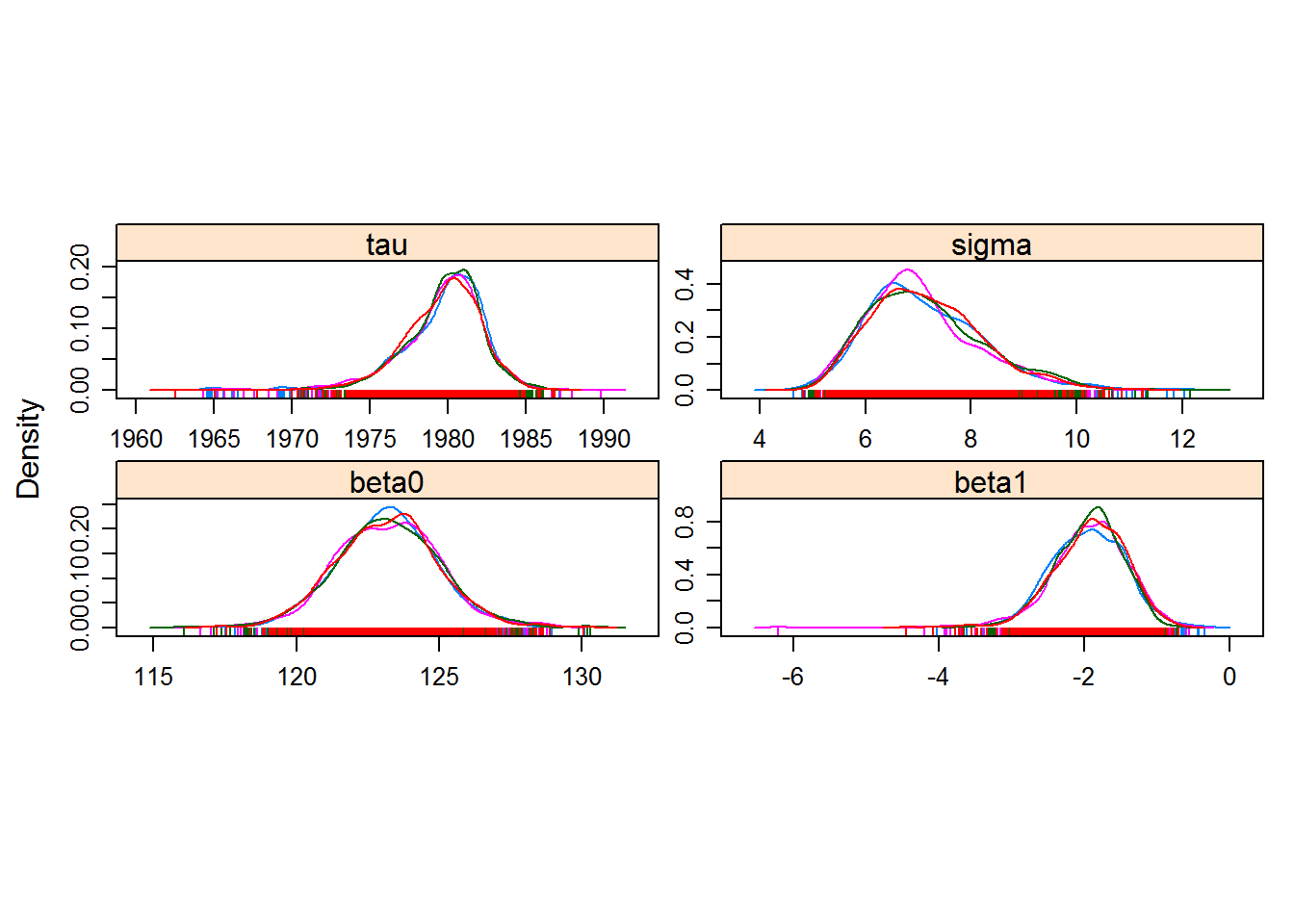
Great fits, nicely behaved chains. And you can see how the final distributions are pretty normal in the end.
The conclusion is that there was likely a structural change in the blooming of this lilac time series occuring somewhere around 1980 (between 1974 and 1984 for sure).
We can see what the point estimate of this model fit might look like, using the getX.hat() function above:
getX.hat <- function(T, beta0, beta1, tau)
  ifelse(T < tau, beta0, beta0 + beta1 * (T-tau))

plot(BLOOM ~ YEAR, pch=19, col=rgb(0,0,0,.5), cex=2, data = l1)
(p.hat <- summary(hockeystick.mcmc)$quantiles[,"50%"])
## beta0 beta1 tau sigma
## 123.208922 -1.908290 1980.119185 6.971224lines(1950:2000, getX.hat(1950:2000, p.hat['beta0'], p.hat['beta1'], p.hat['tau']), lwd=2, col="darkred")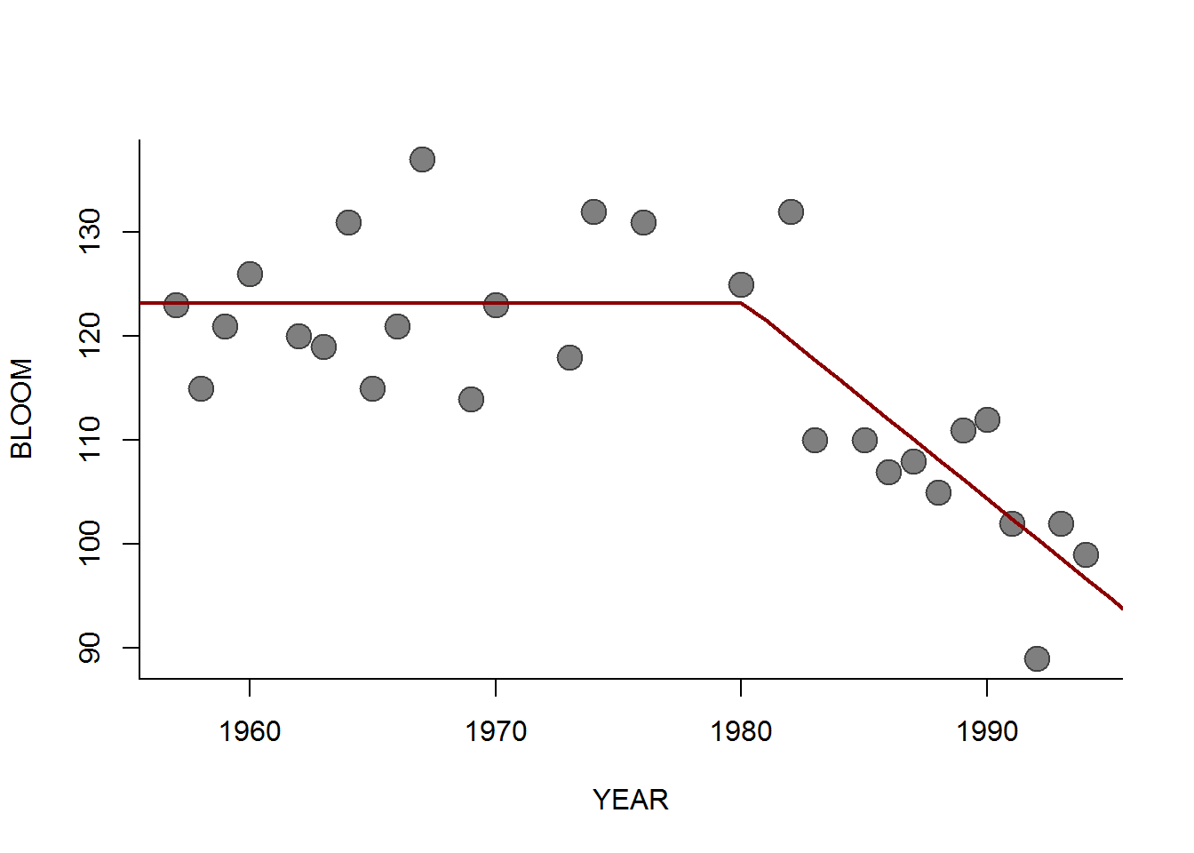
A nice fit. You could also sample from the MCMC results to draw a 95% prediction interval around the time series, though that is a bit trickier to do compactly. Something like this:
par(bty="l")

hockeystick.chains <- as.array(hockeystick.mcmc)
years <- 1950:2000
hockey.sims <- matrix(0, nrow=length(years), ncol=100)
for(i in 1:100)
{
  b0 <- sample(hockeystick.chains[,"beta0",], 1)
  b1 <- sample(hockeystick.chains[,"beta1",], 1)
  tau <- sample(hockeystick.chains[,"tau",], 1)
  hockey.sims[,i] <- getX.hat(years, b0, b1, tau)
}

CIs <- apply(hockey.sims, 1, quantile, p=c(0.025, 0.5, 0.975))

plot(BLOOM ~ YEAR, pch=19, col=rgb(0,0,0,.5), cex=2, data = l1)
lines(years, CIs[1,], col="red", lwd=2, lty=3)
lines(years, CIs[2,], col="red", lwd=2)
lines(years, CIs[3,], col="red", lwd=2, lty=3)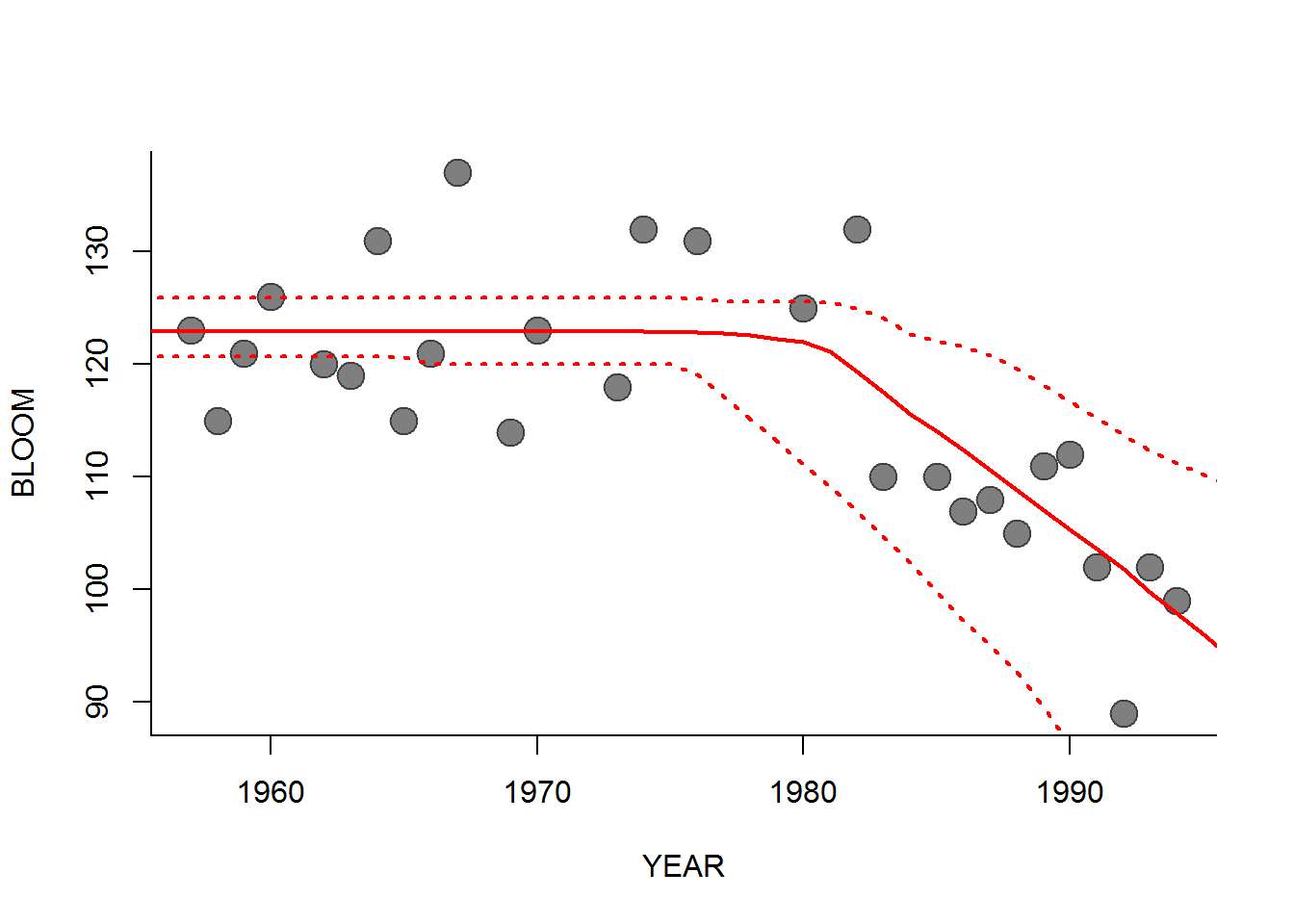
Brief Aside: nonlinear least squares fit
There is a way to fit the “hockey-stick” model to these data using the non-linear least squares nls function in R. Compare the output of the MCMC to these results:
lilacs.nls <- nls( BLOOM ~ getX.hat(YEAR, beta0, beta1, tau),
                   start=list(beta0=120, beta1=-2,tau=1980),
                   data = l1)
summary(lilacs.nls)
##
## Formula: BLOOM ~ getX.hat(YEAR, beta0, beta1, tau)
##
## Parameters:
## Estimate Std. Error t value Pr(>|t|)
## beta0 123.1875 1.7183 71.691 < 2e-16 ***
## beta1 -1.9555 0.5356 -3.651 0.00121 **
## tau 1980.1831 2.6049 760.182 < 2e-16 ***
## ---
## Signif. codes: 0 '***' 0.001 '**' 0.01 '*' 0.05 '.' 0.1 ' ' 1
##
## Residual standard error: 6.873 on 25 degrees of freedom
##
## Number of iterations to convergence: 2
## Achieved convergence tolerance: 7.425e-09The nls function fits the curve by minimizing the least squared …
Brief Aside II: … or “handmade” likelihood
… which is the equivalent of fitting a model with a Gaussian error, which we can also do by obtating an MLE. The likelihood function is:
hockeystick.ll <- function(par, time, x){
    x.hat <- getX.hat(time, par["beta0"], par["beta1"], par["tau"])
    residual <- x - x.hat
    -sum(dnorm(residual, 0, par["sigma"], log=TRUE))
}

par0 <- c(beta0 = 120, beta1 = -2, tau=1980, sigma = 7)
fit.ll <- optim(par0, hockeystick.ll, time = l1$YEAR, x = l1$BLOOM)
fit.ll$par
## beta0 beta1 tau sigma
## 120.437179 -2.133036 1981.999999 6.427344Brief pro-tip … since \(\sigma\) is positive, you’re almost always better off estimating \(\log(\sigma)\), e.g.
hockeystick.ll <- function(par, time, x){
    x.hat <- getX.hat(time, par["beta0"], par["beta1"], par["tau"])
    residual <- x - x.hat
    -sum(dnorm(residual, 0, exp(par["logsigma"]), log=TRUE))
}

par0 <- c(beta0 = 120, beta1 = -2, tau=1980, logsigma = 1)
fit.ll <- optim(par0, hockeystick.ll, time = l1$YEAR, x = l1$BLOOM)
fit.ll$par
## beta0 beta1 tau logsigma
## 123.266231 -1.976351 1980.347135 1.862857“Better off” - in this case - meaning: fewer errors and a faster solution. Also - it’s a quick way to provide the common bound: \([0,\infty]\). The estimate, in the end, is the same:
exp(fit.ll$par['logsigma'])## logsigma
## 6.4421175. Hierarchical hockey stick model
Lets now try to fit a hierarchical model, in which we want to acknowledge that there are lots of sites and variability across them, and we want to see how variable the main timing parameters (flat intercept - \(\beta_0\), decreasing slope - \(\beta_1\)) are across locations.
In this hierarchical model, we specify several are wide distributions for the site-specific parameters, thus:
\[Y_{ij} = f(X_j | \beta_{0,i}, \beta_{1,i}, \tau, \sigma)\]
Where \(i\) refers to each site, and \(j\) refers to each year observation.
\[ \beta_0 \sim {\cal N}(\mu_{\beta 0}, \sigma_{\beta 0}); \beta_1 \sim {\cal N}(\mu_{\beta 1}, \sigma_{\beta 1})\]
We now have 6 parameters, the mean and standard deviation across all sites for two parameters and the overall change point and variance.
STAN code for hierarchical hockeysticks
The complete STAN code to fit this model is below:
data {
  int<lower=0> n;                     // number of total observations
  int<lower=1> nsites;                // number of sites
  int<lower=1,upper=nsites> site[n];  // vector of site IDs
  real y[n];                        // flowering date
  real x[n];                        // year
}

parameters {
  real mu_beta0;  // mean intercept
  real<lower=0> sd_beta0;  // s.d. of intercept

  real mu_beta1;  // mean slope
  real<lower=0> sd_beta1;  // s.d. of intercept

  // overall changepoint and s.d.
  real<lower = min(x), upper = max(x)> tau;
  real<lower=0> sigma;

  vector[nsites] beta0;
  vector[nsites] beta1;
}

model {
  vector[n] yhat;

  // Priors
  sigma ~ inv_gamma(0.001, 0.001);
  mu_beta0 ~ normal(150,150);
  sd_beta0 ~ inv_gamma(0.001, 0.001);
  mu_beta1 ~ normal(0, 10);
  sd_beta1 ~ inv_gamma(0.001, 0.001);
  tau ~ uniform(min(x), max(x));

  for (i in 1:nsites){
    beta0[i] ~ normal(mu_beta0, sd_beta0);
    beta1[i] ~ normal(mu_beta1, sd_beta1);
  }

 // The model!
  for (i in 1:n)
    yhat[i] = beta0[site[i]] + int_step(x[i]-tau) * beta1[site[i]] * (x[i] - tau);

  // likelihood / probability model
  y ~ normal(yhat, sigma);
}
Several things to note here:
The
datamodule now includes a vector of site locationssite, and an extra important variablensitesthat is simply the number of unique sites.- The
parametermodule include the parameters above, but will also keep track of the individualbeta0andbeta1values that are estimated [at no extra cost] for each site. The
modelmodule specifies that the values of the paramters in each site are drawn from the normal distributions, and then obtains the mean function (yhat) referencing the parameter values that are particular to each site.
The STAN code here is saved under the filename hhs.stan.
Compile:
hhs_stan <- stan_model(file = "./_stanmodels/hhs.stan")Selecting sites
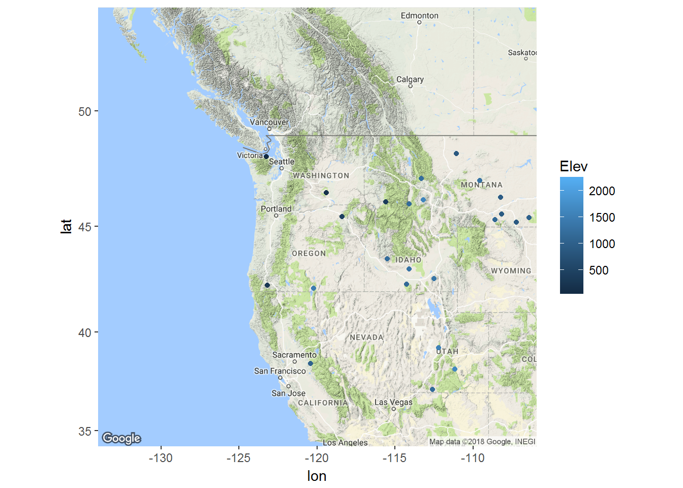
Let’s randomly pick out 30 sites with the most observations (e.g. at least 20), and plot them:
# only lilacs, non NA
lp2 <- subset(lp, !is.na(BLOOM) & SPECIES == 2)
somestations <- names(which(table(lp2$STATION)>20)) %>% sample(30)
lilacs <- subset(lp2, STATION %in% somestations) %>%
      merge(ll, by.x = "STATION", by.y = "ID")
A map:
Running the sampler
First, we have to define the data, recalling that every declared bit of data in the original data module must be present:
Data <- with(lilacs, list(x = YEAR, y = BLOOM, n = length(YEAR),
              site = STATION %>% factor %>% as.integer,
                          nsites = length(unique(STATION))))
These data are longer - in my sample of sites, there are over 700 rows. ALso, the model is more complex and the sampling will take more time, so for now I only do 2 chains.
load(file="./_stanmodels/hhs.stanmodel")
hhs.fit <- sampling(hhs_stan, Data, iter = 2000, chains = 2)
##
## SAMPLING FOR MODEL 'hierarchicalhockeystick' NOW (CHAIN 1).
##
## Chain 1, Iteration: 1 / 2000 [ 0%] (Warmup)
## Chain 1, Iteration: 200 / 2000 [ 10%] (Warmup)
## Chain 1, Iteration: 400 / 2000 [ 20%] (Warmup)
## Chain 1, Iteration: 600 / 2000 [ 30%] (Warmup)
## Chain 1, Iteration: 800 / 2000 [ 40%] (Warmup)
## Chain 1, Iteration: 1000 / 2000 [ 50%] (Warmup)
## Chain 1, Iteration: 1001 / 2000 [ 50%] (Sampling)
## Chain 1, Iteration: 1200 / 2000 [ 60%] (Sampling)
## Chain 1, Iteration: 1400 / 2000 [ 70%] (Sampling)
## Chain 1, Iteration: 1600 / 2000 [ 80%] (Sampling)
## Chain 1, Iteration: 1800 / 2000 [ 90%] (Sampling)
## Chain 1, Iteration: 2000 / 2000 [100%] (Sampling)#
## # Elapsed Time: 4.057 seconds (Warm-up)
## # 3.305 seconds (Sampling)
## # 7.362 seconds (Total)
## #
## [1] "The following numerical problems occurred the indicated number of times on chain 1"
## count
## Exception thrown at line 48: normal_log: Scale parameter is 0, but must be > 0! 1
## [1] "When a numerical problem occurs, the Hamiltonian proposal gets rejected."
## [1] "See http://mc-stan.org/misc/warnings.html#exception-hamiltonian-proposal-rejected"
## [1] "If the number in the 'count' column is small, there is no need to ask about this message on stan-users."
##
## SAMPLING FOR MODEL 'hierarchicalhockeystick' NOW (CHAIN 2).
##
## Chain 2, Iteration: 1 / 2000 [ 0%] (Warmup)
## Chain 2, Iteration: 200 / 2000 [ 10%] (Warmup)
## Chain 2, Iteration: 400 / 2000 [ 20%] (Warmup)
## Chain 2, Iteration: 600 / 2000 [ 30%] (Warmup)
## Chain 2, Iteration: 800 / 2000 [ 40%] (Warmup)
## Chain 2, Iteration: 1000 / 2000 [ 50%] (Warmup)
## Chain 2, Iteration: 1001 / 2000 [ 50%] (Sampling)
## Chain 2, Iteration: 1200 / 2000 [ 60%] (Sampling)
## Chain 2, Iteration: 1400 / 2000 [ 70%] (Sampling)
## Chain 2, Iteration: 1600 / 2000 [ 80%] (Sampling)
## Chain 2, Iteration: 1800 / 2000 [ 90%] (Sampling)
## Chain 2, Iteration: 2000 / 2000 [100%] (Sampling)#
## # Elapsed Time: 10.803 seconds (Warm-up)
## # 115.774 seconds (Sampling)
## # 126.577 seconds (Total)
## #Note that the output of hhs.fit shows estimates for the seven parameters of interest, as well as values of the three parameters for EACH site. We won’t show those here, but here are the main ones:
print(hhs.fit, pars = c("mu_beta0", "sd_beta0", "mu_beta1","sd_beta1", "tau", "sigma"))## Inference for Stan model: hierarchicalhockeystick.
## 2 chains, each with iter=2000; warmup=1000; thin=1;
## post-warmup draws per chain=1000, total post-warmup draws=2000.
##
## mean se_mean sd 2.5% 25% 50% 75% 97.5%
## mu_beta0 127.63 0.09 4.01 119.73 124.87 127.63 130.25 135.58
## sd_beta0 20.82 0.07 2.94 15.99 18.79 20.50 22.48 27.54
## mu_beta1 -0.84 0.02 0.25 -1.28 -1.02 -0.88 -0.67 -0.36
## sd_beta1 0.16 0.05 0.17 0.00 0.02 0.10 0.24 0.61
## tau 1980.69 0.31 3.14 1973.06 1979.89 1981.99 1982.69 1983.75
## sigma 8.88 0.01 0.23 8.46 8.72 8.87 9.03 9.34
## n_eff Rhat
## mu_beta0 2000 1.00
## sd_beta0 2000 1.00
## mu_beta1 113 1.02
## sd_beta1 12 1.26
## tau 100 1.02
## sigma 2000 1.00
##
## Samples were drawn using NUTS(diag_e) at Fri Jan 19 13:36:02 2018.
## For each parameter, n_eff is a crude measure of effective sample size,
## and Rhat is the potential scale reduction factor on split chains (at
## convergence, Rhat=1).Visualiziaing the chains:
hhs.mcmc <- As.mcmc.list(hhs.fit, pars = c("mu_beta0", "sd_beta0", "mu_beta1","sd_beta1", "tau",  "sigma"))
xyplot(hhs.mcmc)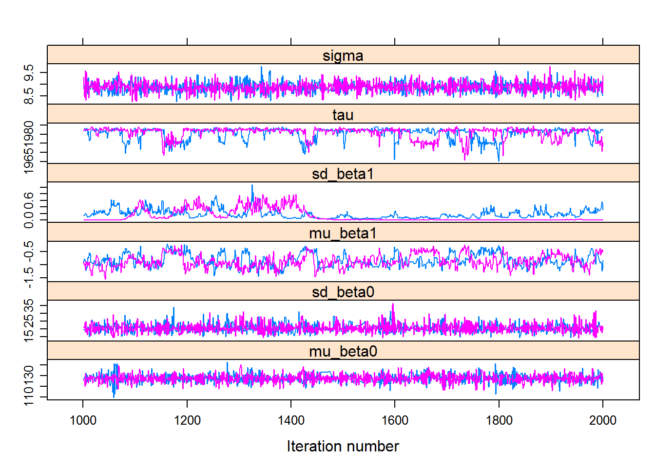
densityplot(hhs.mcmc)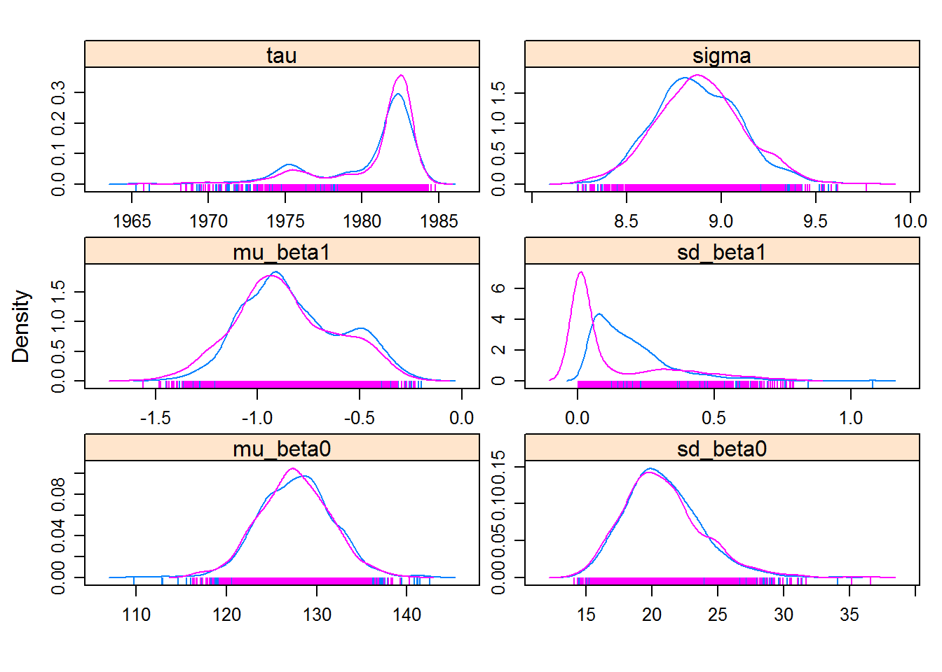
You might (depending on your specific results) see that the question of “convergence” is a little bit more open here. But certainly the wide variation in the mean intercept \(\beta_0\) is notable, as is the uniformly negative slope \(\beta_1\).
6. Hierarchical hockeystick … with covariates
We’re going to do one more twist on the model, and that is to try to narrow the rather large variation in the intercept by using our latitude and longitude information. In this model, the intercept (\(\beta_0\)) will be explained by elevation and latitude - the higher and further north you are, the more later flowers tend to bloom. So in this model, everyting will be the same as above, except that rather than have \(\beta_0 \sim {\cal N}(\mu, \sigma)\) - it is going to be a regression model:
\[\beta_0 \sim {\cal N}({\bf X} \beta, \sigma)\]
where \({\bf X}\) represents a design matrix of the form:
\[\left[\begin{array}{ccc} 1 & E_1 & L_1 \\ 1 & E_2 & L_2 \\ 1 & E_3 & L_3 \\ ... & ... & ...\\ \end{array}\right]\]
where \(E\) and \(L\) represent elevation and latitude.
Coding this adds a few quirks to the STAN code, but surprisingly not many more lines. See the complete code here: https://terpconnect.umd.edu/~egurarie/teaching/Biol709/stanmodels/hhswithcovar.stan.
## hhswc_stan <- stan_model("hhswithcovar.stan")A quick way to get a covariate matrix below. Note that I center the covariates, so that the intercept is the mean value, and the slopes tell me the number of days PER degree latitude and PER 1 km elevation:
covars <- with(lilacs, model.matrix(BLOOM ~ I(Lat - mean(Lat)) + I((Elev - mean(Elev))/1000)))
head(covars)
## (Intercept) I(Lat - mean(Lat)) I((Elev - mean(Elev))/1000)
## 1 1 -4.406203 -0.08824224
## 2 1 -4.406203 -0.08824224
## 3 1 -4.406203 -0.08824224
## 4 1 -4.406203 -0.08824224
## 5 1 -4.406203 -0.08824224
## 6 1 -4.406203 -0.08824224Which we now include in our Data list:
Data <- with(lilacs,
            list(x = YEAR, y = BLOOM, n = length(YEAR),
               site = STATION %>% factor %>% as.integer,
                          nsites = length(unique(STATION)),
                          covars = covars, ncovars = ncol(covars)))
And sample:
hhswc.fit <- sampling(hhswc_stan, Data, chains = 4, iter = 2000)pars <- names(hhswc.fit)[1:8]
hhswc.mcmc <- As.mcmc.list(hhswc.fit, pars)
summary(hhswc.mcmc)##
## Iterations = 1001:2000
## Thinning interval = 1
## Number of chains = 4
## Sample size per chain = 1000
##
## 1. Empirical mean and standard deviation for each variable,
## plus standard error of the mean:
##
## Mean SD Naive SE Time-series SE
## mu_beta0[1] 125.4290 1.41959 0.022446 0.073132
## mu_beta0[2] 3.5104 0.44462 0.007030 0.011745
## mu_beta0[3] 31.6962 2.33492 0.036918 0.136656
## sd_beta0 2.0718 0.33017 0.005220 0.014048
## mu_beta1 -0.5536 0.12199 0.001929 0.006485
## sd_beta1 0.1968 0.08792 0.001390 0.005424
## tau 1975.9873 1.81555 0.028706 0.084441
## sigma 8.3531 0.21720 0.003434 0.003210
##
## 2. Quantiles for each variable:
##
## 2.5% 25% 50% 75% 97.5%
## mu_beta0[1] 122.55436 124.4969 125.4511 126.3495 128.2263
## mu_beta0[2] 2.58726 3.2265 3.5225 3.8032 4.3729
## mu_beta0[3] 26.88464 30.1903 31.7624 33.2996 35.9938
## sd_beta0 1.53432 1.8393 2.0316 2.2705 2.8162
## mu_beta1 -0.87583 -0.6116 -0.5398 -0.4741 -0.3606
## sd_beta1 0.03615 0.1347 0.1949 0.2534 0.3851
## tau 1973.14730 1974.9176 1975.5641 1976.7091 1980.7888
## sigma 7.94052 8.2023 8.3525 8.5028 8.7784xyplot(hhswc.mcmc)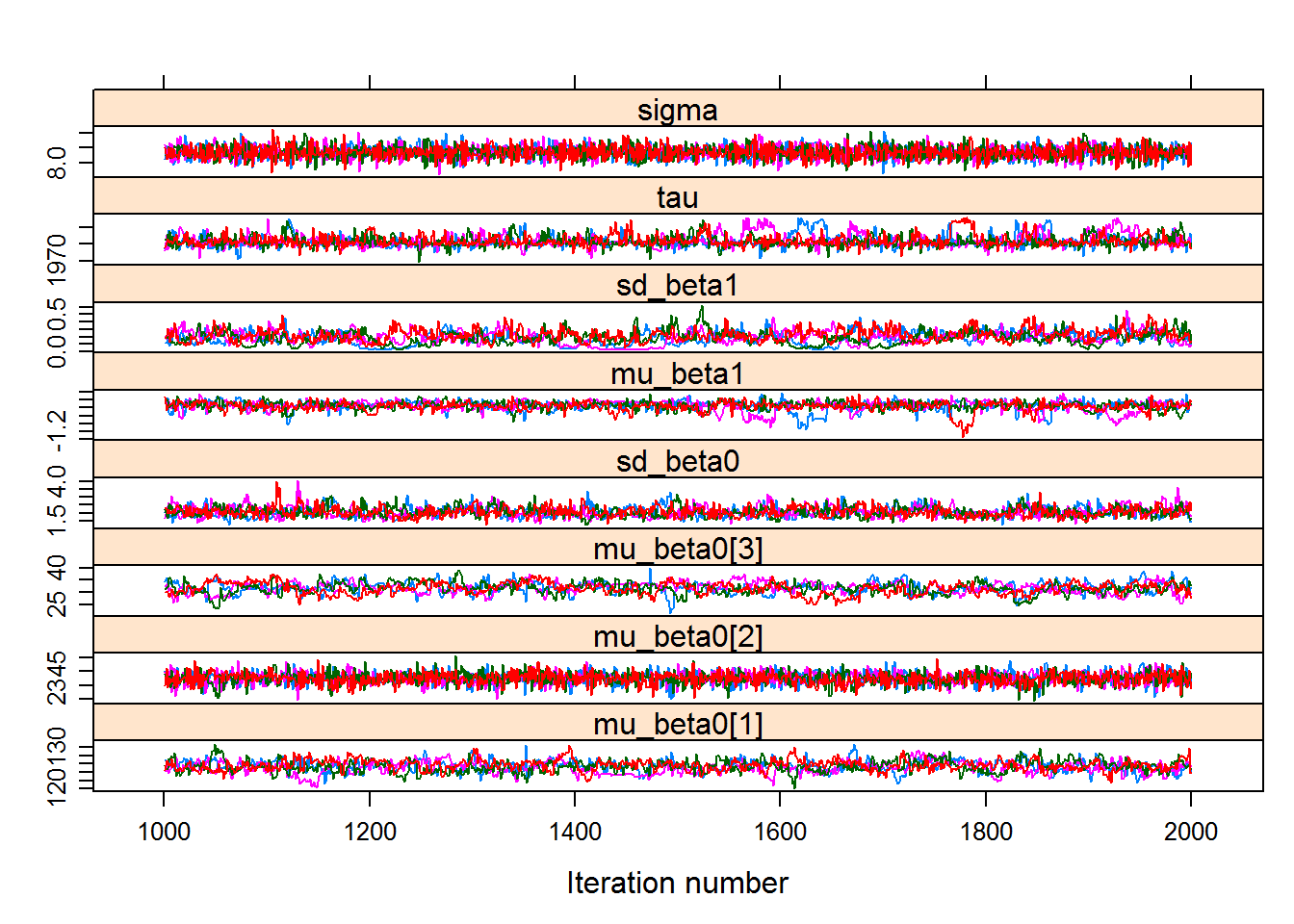
densityplot(hhswc.mcmc)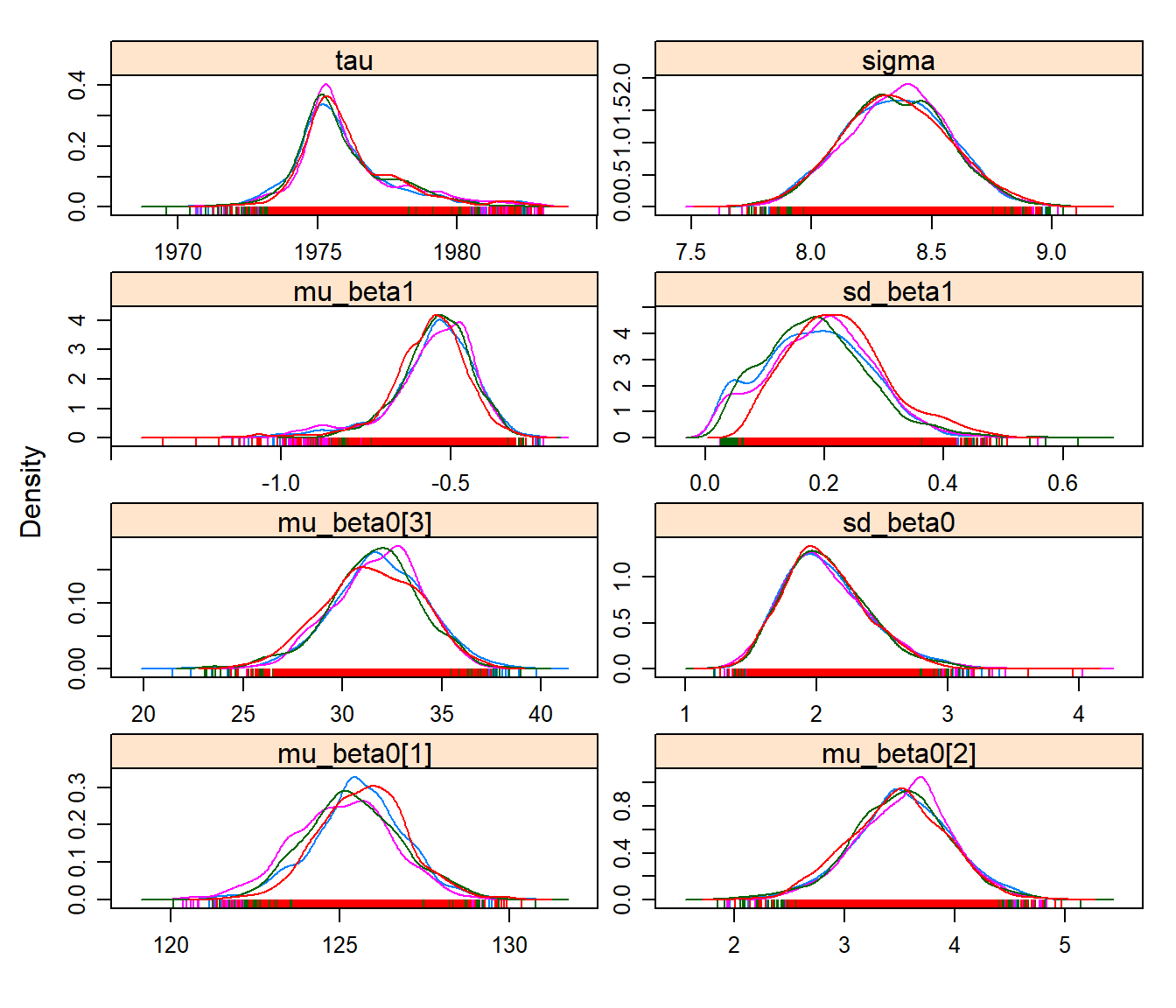
Note that this model provides much more consistent, converging results! This is because more data were leveraged, and the response is clearly a strong one. The “base” mean day was around 136, the latitude effect is about +3.74 days per degree latitude, and the elevation effect is about +30 days for every 1000 m. The slope is still significantly negative, and the mean transition year is somewhere in the early-mid 70’s.