I. Bayesian Basics
BIOL709/BSCI339
Bayesian Inference
… (the good nutshell)
is according to some a radically different and modern approach to modeling data that:
- assumes (a priori) that parameters are not fixed, unknown, painstakingly inferred, constants but UNCERTAIN/RANDOM
- allows you to incorporate PRIOR information about those parameters …
- by letting DATA “update” your prior belief.
- allows you to estimate models with a high PARAMETER/DATA ratio (even >1!),
- or that are way more complex and hierarchical than feasible in any other way,
- while staying (arguably) closer to how humans (and animals) cognitively model the world
(the bad nutshell)
according to others
- is logically suspicious
- unacceptably subjective
- overly computationally intensive
- hideously dependent on post-hoc processing of “chains”
More than anything, Bayesian inference …
… provides the best excuse in 150 years for statisticians/analysts to polarize into antagonistic camps (frequenists vs. Bayesianists) and engage in (often, in my opinion) pointless, pedantic, pseudo-philosophical arguments.

How does it do all these things?
We have to go back to some basic definitions in PROBABILITY THEORY.
Conditional probability
hair & eye color:
(HE <- HairEyeColor[,,2] + HairEyeColor[,,1])## Eye
## Hair Brown Blue Hazel Green
## Black 68 20 15 5
## Brown 119 84 54 29
## Red 26 17 14 14
## Blond 7 94 10 16(HE.p <- round(prop.table(HE),3))## Eye
## Hair Brown Blue Hazel Green
## Black 0.115 0.034 0.025 0.008
## Brown 0.201 0.142 0.091 0.049
## Red 0.044 0.029 0.024 0.024
## Blond 0.012 0.159 0.017 0.027What’s the probability of event A given event B.
\[\text{Pr}(A|B)\]
e.g.: \[Prob(Eye = blue | Hair = blond)\]
How do you compute this?
\(Pr(Eyes = blue \& Hair = blond) = 0.159\)
##        Eye
## Hair    Brown  Blue Hazel Green
##   Black 0.115 0.034 0.025 0.008
##   Brown 0.201 0.142 0.091 0.049
##   Red   0.044 0.029 0.024 0.024
## Blond 0.012 0.159 0.017 0.027\(Pr(Hair = blond) = 0.215\)
rowSums(HE.p)## Black Brown Red Blond
## 0.182 0.483 0.121 0.215\[\text{Pr}(A|B) = {Pr(A, B) \over Pr(B)}\]
Probability of having blue eyes given that your hair is blond:
HE.p[4,2]/rowSums(HE.p)[4]## Blond
## 0.7395349Very High!
Compare to overall probability of blue eyes.
Are Conditional Probabilities Symmetric?
\[\text{Pr}(A|B) = \text{Pr}(B|A)?\]
Blond haired given you’re blue eyed:
HE.p[4,2]/colSums(HE.p)[2]## Blue
## 0.4368132Obviously not! But what is the relationship?
Bayes Theorem
\[\text{Pr}(A|B) = {\text{Pr}(B|A) P(A) \over P(B)}\]
Straightforward, non-controvertial, fundamental law of probabilities:
“Bayes’ theorem is to the theory of probability what Pythagoras’s theorem is to geometry.” - Harold Jeffreys
Simple - but not always intuitive
Consider a disease (e.g. ebola) that exists with a prevalance of 0.0001 in the population: \[P(E) = 0.0001\]
There is a test, which has a 99% positive identification rate, i.e. if you DO have ebola, a positive result has probability 0.99: \[P(+|E) = 0.99\]
The test also has a 1% false positive rate, i.e. if you DON’T have ebola, the result will be negative. \[P(+|!E) = 0.01\]
YOU test positive! What’s the probability you have ebola?
Probabilities:
\[P(E) = 1e(-4)\] \[P(+|E) = 0.99\] \[P(+| !E) = 0.01\]
Simple - but not always intuitive
Probabilities:
\[P(E) = 1e(-4)\] \[P(+|E) = 0.99\] \[P(+| !E) = 0.05\]
\[P(E|+) = {P(+|E) P(E) \over P(+)}\]
\[P(E|+) = {P(+|E) P(E) \over (P(+|!E) P(!E) + P(+|E) P(E)}\]
\[P(E|+) = {0.99 \times 1e(-4) \over 0.99 \times 1e(-4) + 1e(-2) \times (1 - 1e(-4)}\] \[P(E|+) \approx {1e-4 \over 1e-4 + 1e-2}\] \[P(E|+) \approx 0.0099\]
Perhaps … lower than you expected?
From Bayes’ Theorem to Bayesian Inference
Bayes Theorem:
\[\text{Pr}(A|B) = {\text{Pr}(B|A) P(A) \over P(B)}\]
where: \(A\) - is anything and \(B\) - is anything
Bayesian Inference:
\[\pi(\theta | {\bf X}) = {p({\bf X} | \theta) \pi (\theta) \over p({\bf X})}\]
where: \({\bf X}\) - is DATA and \({\theta}\) - is parameters
Shockingly (or intuitively?) PARAMETERS are random!?
The goal is to obtain a probability distribution of parameter values given data:
- \(\pi(\theta|X)\) - posterior distribution)
basing that inference by adjusting a “naive” guess:
- \(\pi(\theta)\) - prior distribution)
by multiplying (updating):
- \(p(X|\theta)\) - probability of data given parameters
What is this thing called?
Yes! the Likelihood!
\[\pi(\theta | {\bf X}) = {p({\bf X} | \theta) \pi (\theta) \over p({\bf X})}\]
In the ebola example, we want to infer the parameter \(p_{you\,have\,ebola}\).
The prior: \(\pi(\theta) = Pr(E) = p_{ebola\,in\,population}\).
The data: \({\bf X} = +\)
The likelihood: \(p({\bf X} | \theta) = P(+|E)\)
The updating of the prior: \(p({\bf X} | \theta) \pi(\theta) = P(+|E) P(E)\)
The normalizing of the prior: \[p(X) = \int_{\theta} p(X|\theta^*) \pi(\theta^*) d\theta^*\] \[= P(+|!E) P(!E) + P(+|E) P(E)\]
Note: this normalization is - here and in other cases - the biggest pain! But thankfully, also, not always necessary.
In words:
We took the very strong prior probability distribution \(p_{you\,have\,ebola} = 0.0001\) and “nudged” it with our new, slightly imperfect observation to \(p_{you\,have\,ebola} = 0.01\).
Bayes Theorem (redacted):
\[\pi(\theta | {\bf X}) \propto p({\bf X} | \theta) \pi (\theta)\]
- Everything is based on having a prior (a priori) idea of the parameters!
- From a frequentist perspective, it is ABSURD to talk about the \(\pi(\theta)\) - since that is assumed to be a fixed, unknown quantity… There is only an ESTIMATE
- The biggest bugaboo of Bayes is in determining the prior distribution. What should the prior be? What influence does it have?
- The expression above is not an equality - but no matter because it is a distribution that can be normalized. The missing demonimator is \(p({\bf X})\) is often a very difficult thing to compute.
The Goal:
Is (always) to compute the posterior distribution of the parameters: \(\pi(\theta | {\bf X})\)
What does that mean for a distribution? What are point estimates? How do we quantify uncertainty?
There are options!
A point estimate can be the mean of the posterior: \(\widehat{\theta} = E(\theta | {\bf X}) = \int \theta \pi(\theta|{\bf X})\, d\theta\),
or median or mode.
Uncertainty is given by a Credible Interval, i.e. \(a\) and \(b\) such that: \(\int_a^b \pi(\theta|{\bf X}) = 1 - \alpha\)
You are allowed to interpret this as the Probability of a parameter being within this interval! (to the great relief of statistics students who are understanably confused about the interpretation of Confidence Intervals).
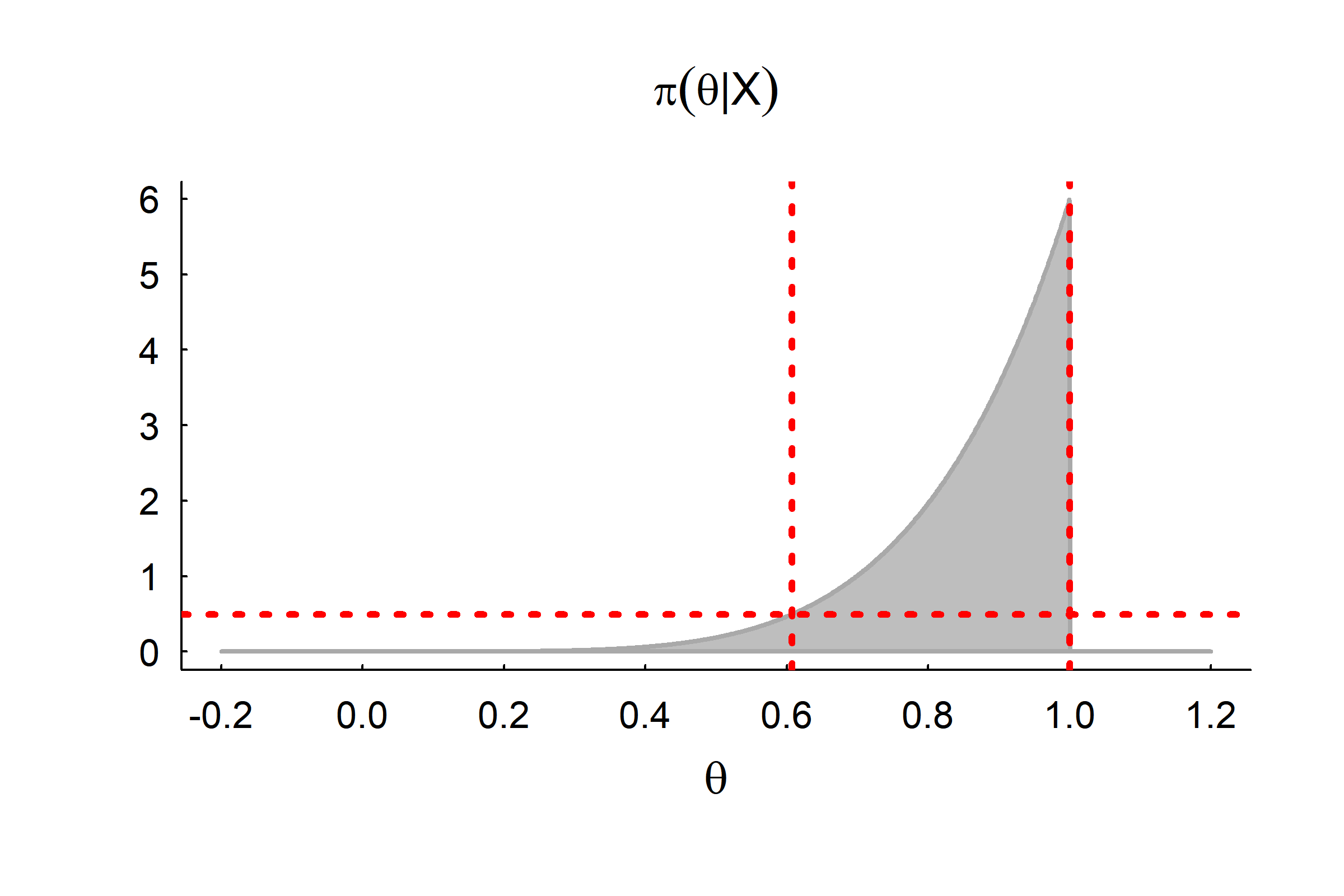
Example: Coin Toss (uniform prior)
Data: \[{\bf X} = \{H,H,H,H,H\}\]
Uninformative prior: \[\theta \sim \text{Unif}(0,1)\] \[\pi(\theta) = 1; 0 < \theta < 1\]
Likelihood: \[X \sim \text{Binomial}(n=5,\theta)\] \[f(X|\theta) = \theta^5\]
Posterior: \[\pi(\theta|X) \propto 1 \times \theta^5 = 6 \theta^5\]
fillcurve <- function(dist, min=-.2, col="grey", bor=1, lwd =2, max=1.2, n=1e5, ...){
  x <- c(min, seq(min, max, length=1000), max)
  y <- c(0, dist(seq(min, max, length=1000)), 0)
  plot(x, y, type="n", ylab="",...)
  polygon(x, y, col=col, bor=bor, lwd=lwd)
}
pi1 <- function(theta) ifelse(theta >= 0 & theta <= 1, 6*theta^5, 0)
fillcurve(dunif, xlab=expression(theta), main="Prior")
fillcurve(pi1, xlab=expression(theta), main="Posterior")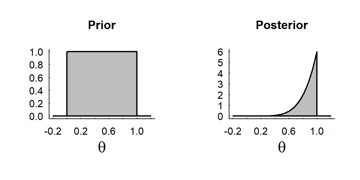
Point Estimation
With this new posterior distribution we can report some results with respect to our parameter!
Mean: \[\widehat{\theta} = \int_0^1 \theta \times 6 \theta^5 d\theta = 6/7 = 0.857\]
Median: \[\tilde{\theta}: \int_0^{\tilde{\theta}} 6 \theta^5 d\theta = 1/2\] \[ \tilde{\theta}^6 = {1 \over 2}; \tilde{\theta} = {1 \over 2}^{1/6} = 0.89\]
Mode: \[\breve{\theta} = \text{argmax}_\theta (f(\theta)) = 1\]
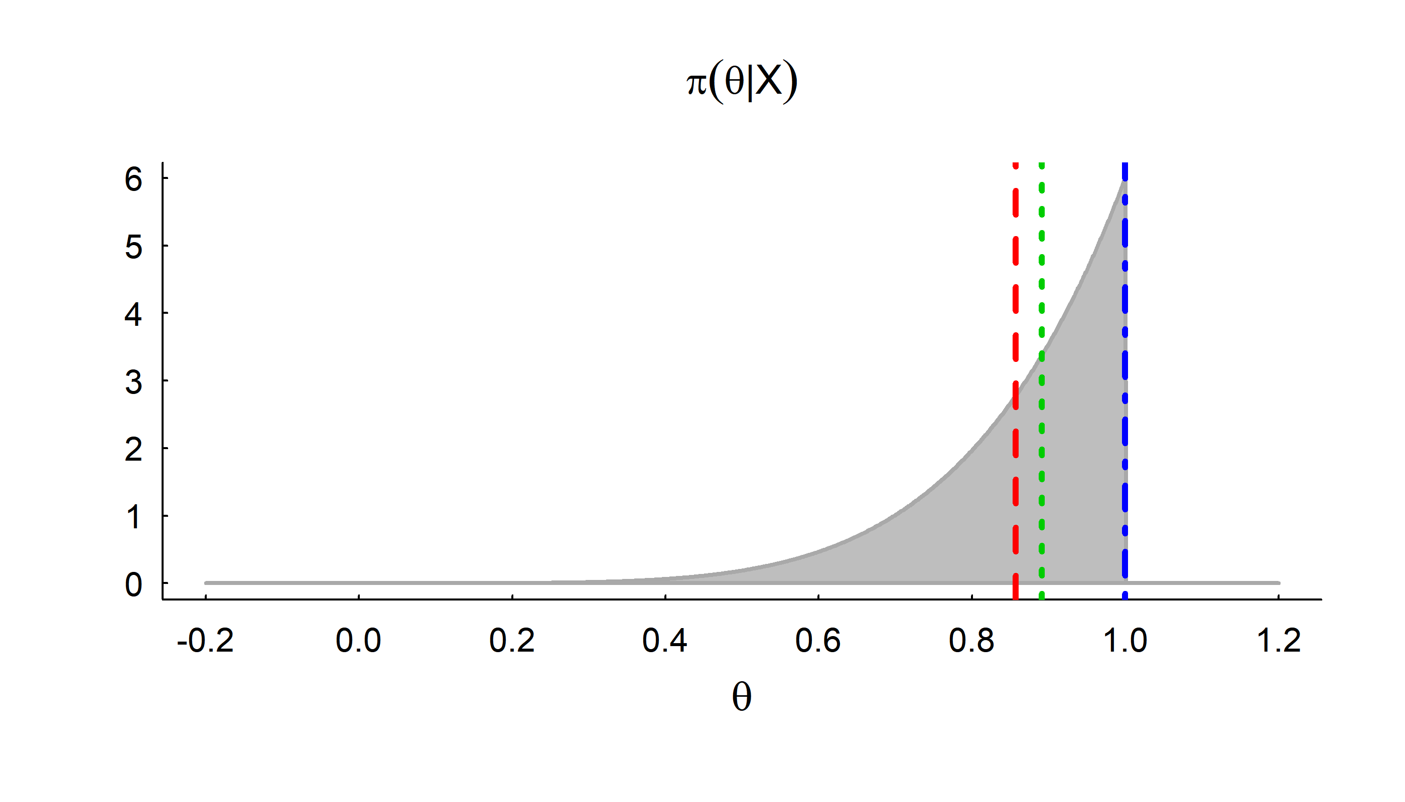
Credible Intervals
95% Central:
\[\int_0^{\{a,b\}} \pi(\theta|X) d\theta = \{0.025, 0.975\}\]
Here: \(a^6 = 0.025;\,\, a = 0.54; b^6 = 0.975;\,\, b = 0.996\)
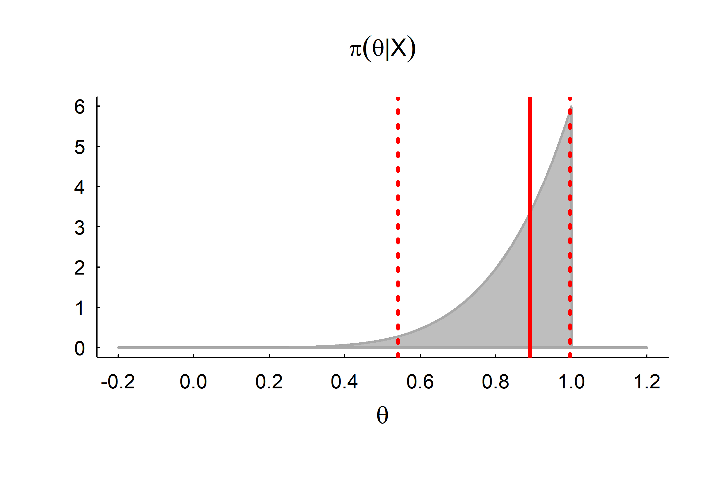
95% Flat top interval:
\(a\) and \(b\) such that \(\pi(a) = \pi(b)\) and \[\int_a^b \pi(\theta|X) d\theta = 0.95\]
Here: \[ 0.607 - 1.0 \]
Comparison to Frequentist Analysis

MLE of \(\widehat{\theta}_{mle} = 1\), but C.I. = 0!?
Bayes allows you to quantify your belief in the parameter’s value where a frequentist approach is mostly useless.
This is because you ALREADY had a model. All the data did was “update” it!
This is often amazing to people who first encounter Bayesian modeling - it CAN estimate parameters with VERY HIGH parameter/data ratios.
Example 2: Magic Coin? (informative prior)
Probably - if someone flips a coin you’ll assume that it’s a fair coin. But maybe you’ve heard of “magic” double-headed or double-tailed coins?
Data: \(\{H,H,H,H,H\}\)
Prior: \(\pi(\theta) = \{0, 1/2, 1\}\) with Prob: \(\{.005, .99, .005\}\)
Exercise 1: Compute the posterior.
Exercise 2: How many consecutive coin flips will it take for the subjective probability that it is a 2-headed coin to be creater than the subjective probability that it is a fair coin?
Question: What happens to the posterior if you observe a single tail - even after a long string of heads?
This illustrates that the stronger the initial belief, the harder it is to shift it! Bayesian statistics is therefore a nice model of an adaptive learning process.
Conjugate Priors
Obviously a large part of Bayesian models has to do with picking priors.
The Uniform(0,1) prior for probabilities is, in fact, a special case of a Beta(a,b) distribution. Even more remarkably, the posterior distribution (for a Binomial process), is ALSO a Beta distribution.
\[ \pi(\theta) = \frac{1}{B(\alpha,\beta)} x^{\alpha-1}(1-x)^{\beta-1} \]
Prior: \(\alpha = \beta = 1\); Posterior: \(\alpha = 6\) , \(\beta = 1\) .
We say that the Beta is the conjugate prior for the p parameter in a Binomial distribution. Conjugate priors are VERY HANDY - both mathematically and computationally, and as you parameterize / try to fit Bayesian models, it is good to be aware of them.
- Beta is also conjugal with Geometric and Negative-Binomial (\(p\))
- Gamma with Poisson - (for rate \(\lambda\))
- Normal with … Normal (for the mean \(\mu\))
- Normal and Gamma - for the Precision parameter \(\tau = 1/\sigma^2\), a favorite of Bayesian modelers, possibly due to the above conjugation.
A summary of conjugate priors here: http://www.johndcook.com/conjugate_prior_diagram.html
Computation
The coin problem is a rare analytically tractable one.
If you have a few more parameters, and maybe odd distributions, you might be able to numerically integrate.
But if you have a lot of parameters, this is a near impossble operation to perform!
Thus, though the theory dates to the 1600’s, it has been difficult to implement more broadly … until the developement of Markov Chain Monte Carlo techniques.
