Lab 9b: Bayesian Inference, the numerical approach

Bayes’ theorem

The goal in any Bayesian analsyis is to obtain a posterior distribution from Bayes’ theorem which says: \[\pi(\mu, \sigma | X) \propto p(X|\mu, \sigma) \pi(\mu, \sigma).\] The steps are straightforward: (1) select priors, (2) define the likelihood, (3) multiply [i.e. integrate] the two functions for “all” possible values of the parameters.

Priors

Let’s use uninformative priors. For the mean, one possibility is a uniform distribution over the range of the data, since the mean must be somewhere in that range:
\[\mu \sim \text{Unif}(X_{min}, X_{min})\] \[ \pi(\mu) = {1 \over X_{max} - X_{min}}\] where \(X_{min} \leq \mu \leq X_{max}\).

For \(\sigma\), it is harder to place bounds, but a nice uninformative positive prior can be the exponential:

\[\sigma \sim \text{Exp}(\lambda_0)\] \[\pi(\sigma) = \lambda \exp(-\lambda \sigma)\] where \(\sigma > 0\) and \(\lambda\) is some very small number.

Set these parameters for the priors:

mu.min <- min(X)
mu.max <- max(X)
lambda <- 1e-4

Likelihood function

The likelihood function (as in all of our estimations) is our actual data model, i.e. the normal distribution: \[p({\bf X}|\mu, \sigma) = \prod_{i=1}^n \phi(X_i, \mu, \sigma)\] wher \(\phi\) is the p.d.f. of the normal distribution.

likelihood <- function(x, mu, sigma) prod(dnorm(X, mu, sigma))

Note that we can not be in the “log-likelihood” world which we prefer for maximum likelihood estimation, since we need the actual probability distribution. That said, for larger amounts of data you would need to toggle back and forth between the log and untransformed units, e.g.:

likelihood <- function(x, mu, sigma) exp(sum(dnorm(X, mu, sigma, log=TRUE)))

Integration

Now that we have all the pieces, we need to compute the posterior distribution: \(\pi(\mu, \sigma)\), which is (proportional) simply to the product of the priors and the likelihood at every value of \(\mu\) and \(\sigma\):

getposterior <- function(mu, sigma)  
  likelihood(X, mu, sigma)*dunif(mu, mu.min, mu.max)*dexp(sigma, lambda)

Initialize vectors for the two parameters (at reasonably high resolution):

dmu <- .01; dsigma <- .01
mus <- seq(min(X),max(X), dmu)
sigmas <- seq(dsigma,5, dsigma)

The slickest way to perform the calculation of the posteriors for all values is our friend outer():

posterior <- outer(mus, sigmas, Vectorize(getposterior))

NOTE: this posterior is not normalized! How would we normalize it if we wanted to?

Here is a visualization of the posterior density:

image(mus, sigmas, posterior, ylim=c(0,2), col=topo.colors(200))
persp(mus, sigmas, posterior, border=NA, shade=TRUE, ticktype="detailed")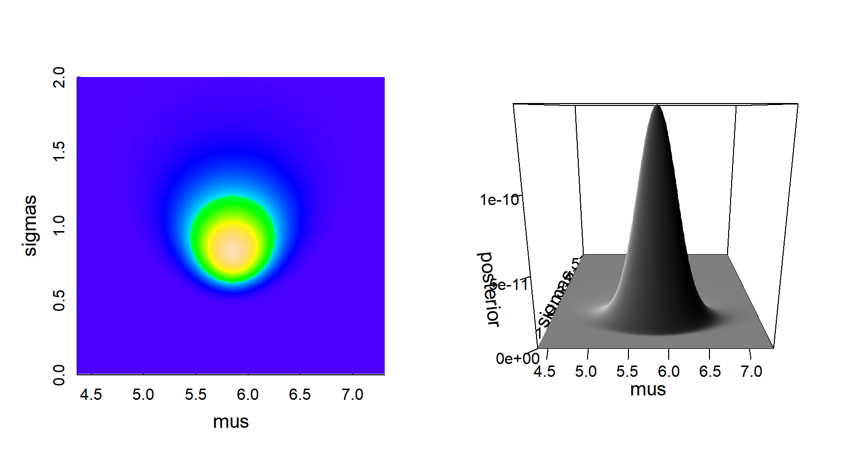

The posterior distribution seems nicely peaked.

Bayesian point estimate

Let’s find the peak (mode) of this distribution, which is one kind of central point estimate of the parameters:

(max.indices <- which(posterior == max(posterior), arr.ind=TRUE))

##      row col
## [1,] 190 118

mu.mode <- mus[max.indices[1]]
sigma.mode <- sigmas[max.indices[2]]

Lets look at the posterior distributions at the maxima, i.e. \(\pi(\mu | \sigma =\widehat\sigma, {\bf X})\) and \(\pi(\sigma | \mu = \widehat{\mu}, {\bf X}\)), and compare it to our prior distributions

mu.post <- posterior[,max.indices[2]] %>% {./sum(.)/dmu}
sigma.post <- posterior[max.indices[1],] %>% {./sum(.)/dsigma}

plot(mus, mu.post, type="l", xlim=range(X) + c(-.5,.5), lwd=2, col="darkgrey")
curve(dunif(x, mu.min, mu.max), add=TRUE, col=2, n=1e5)
legend("topleft", col=c("red", "darkgrey"), legend = c("prior", "posterior"), lty=1, bty="n", lwd=2)

plot(sigmas, sigma.post, type="l", lwd=2, col="darkgrey")
curve(dexp(x, lambda)*1e3, add=TRUE, col=2, n=1e5)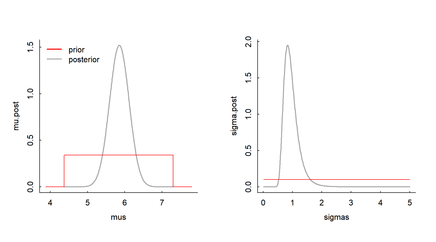

The posteriors are sharper than the priors, meaning the data have successfully “narrowed” the prior towards a useful result.

Credible intervals

A posterior distribution is the complete description of our estimates. But typically, we want to report a point estimate and (e.g.) a 95% credible interval.
To compute these, we need to integrate our posterior and find the location where the cumulative distribution is equal to 0.025 and 0.975, i.e. solve: \[\int_{\theta}^{\{CI_{low}, CI_{high}\}} \pi(\theta|{\bf X}) d\theta = \{0.025, 0.975\}\]

mu.CI.low  <- mus[which.min(abs(cumsum(mu.post)*dmu - 0.025))]
mu.CI.high <- mus[which.min(abs(cumsum(mu.post)*dmu - 0.975))]
sigma.CI.low  <- sigmas[which.min(abs(cumsum(sigma.post)*dsigma - 0.025))]
sigma.CI.high <- sigmas[which.min(abs(cumsum(sigma.post)*dsigma - 0.975))]

Report results:

bayes.fit <- rbind(c(mu.mode, mu.CI.low, mu.CI.high), c(sigma.mode, sigma.CI.low, sigma.CI.high)) %>% data.frame
names(bayes.fit) <- c("mode", "CI.low", "CI.high")
row.names(bayes.fit) <- c("mu", "sigma")
bayes.fit

##       mode CI.low CI.high
## mu    6.69   5.95    7.42
## sigma 1.18   0.85    2.27

Compare to MLE’s

Shall we compare this to the maximum likelihood estimators? These are (analytically solved):

\[\widehat{\mu} = \overline{X} = {1\over n} \sum_{i=1}^n X_i \] \[\widehat{\sigma} = \sqrt{{1 \over n} \sum_{i=1}^n (X_i - \overline{X})^2}\]

(mle.hat <- c(mu = mean(X), sigma = sqrt(sum((X - mean(X))^2)/length(X))))

##       mu    sigma 
## 6.689000 1.182806

We can bootstrap the confidence intervals:

mle.bs <- matrix(NA, 2, 1e4)
for(i in 1:1e4){
  X.resample <- sample(X, replace=TRUE)
  mle.bs[, i] <- c(mu = mean(X.resample), sigma = sqrt(sum((X.resample - mean(X.resample))^2/length(X.resample))))
}
CIs <- apply(mle.bs, 1, quantile, p = c(0.025, 0.975))

(mle.fit <- cbind(mle.hat, t(CIs)))

##        mle.hat      2.5%    97.5%
## mu    6.689000 5.9430000 7.436050
## sigma 1.182806 0.6701629 1.485074

Compare with:

bayes.fit

##       mode CI.low CI.high
## mu    6.69   5.95    7.42
## sigma 1.18   0.85    2.27

The point estimates should be right on for both parameters, and the bootstrapped confidence intervals (maybe: BCI) and Bayesian credible intervals (maybe also: BCI?!) are right on for the means, but might be rather different for the standard deviations.

In both analyses, we can actually visualize the distribution of our estimates:

hist(mle.bs[1,], breaks=50, col="grey", bor="darkgrey", freq=FALSE, xlab="mean", main = "")
lines(mus, mu.post, lwd=2, col=2, xpd=0)

legend("topleft", legend = c("bootstrap", "posterior"), 
       col = c(NA, "red"), pt.bg = c("grey", NA), pch = c(22, NA), pt.cex=2,  lty=c(NA, 1),  bty="n")

hist(mle.bs[2,], breaks=50, col="grey", bor="darkgrey", freq=FALSE, 
     xlim=c(0,2.0), xlab="standard deviation", main="")
lines(sigmas, sigma.post, lwd=2, col=2)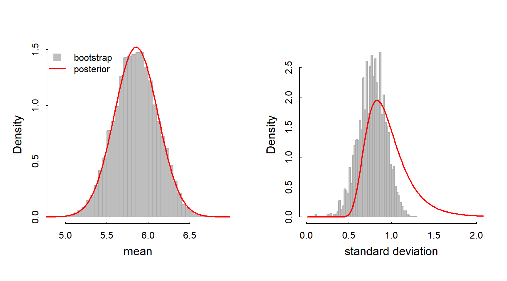

The mean distributions should look quite similar, whereas the bootstrapped distribution around \(\widehat{\sigma}\) might be multimodal, or very skewed, or generally be dissimilar to the posterior. Can you think why this might be? Which of these do you “trust” more?