This simulation
explores the problem of measuring the height of a small peak
(also called a "child peak") that is buried in the tail of a
much stronger overlapping peak (a "parent peak"),
in the especially challenging case that the smaller peak is not even visible to
the unaided eye. Three different measurement tools will be
explored: iterative
least-squares, classical least-squares regression,
and peak detection, using the
Matlab/Octave tools peakfit.m,
cls.m, or findpeaksG.m,
respectively. (Alternatively, you could use the corresponding spreadsheet
templates).
In this example the larger peak is located at x=4 and has a
height of 1.0 and a width of 1.66; the smaller measured peak is
located at x=5 and has a height of 0.1 and also with a width of
1.66. Of course, for the purposes of this simulation, we pretend
that we don't necessarily know all of these facts and we will
try to find methods that will extract such information as
possible from the data, even if the signal is noisy. The
measured peak is small enough and close enough to the stronger
overlapping peak (separated by less than the width of the peaks)
that it never forms a maximum
in the total signal. So 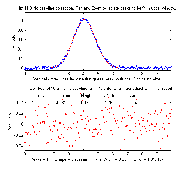 it looks like there is only
one peak, as
shown on the figure on the right. For that reason the
findpeaks.m function (which automatically finds peak maxima)
will not be useful by itself to locate the smaller peak. Simpler
methods for detecting the second peak also fail to provide a way
to measure the smaller second peak, such as inspecting the
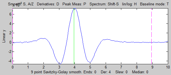
derivatives of the signal (the smoothed fourth derivative shows
some
evidence of asymmetry, but that could just be due to the
shape of the larger peak), or Fourier self-deconvolution to
narrow the peaks so they are distinguishable, but that is
unlikely to be successful with this much noise. Least-squares
methods work better when the signal-to-noise ratio is poor, and they can be fine-tuned to make use of available
information or constraints, as will be demonstrated below.
it looks like there is only
one peak, as
shown on the figure on the right. For that reason the
findpeaks.m function (which automatically finds peak maxima)
will not be useful by itself to locate the smaller peak. Simpler
methods for detecting the second peak also fail to provide a way
to measure the smaller second peak, such as inspecting the
derivatives of the signal (the smoothed fourth derivative shows
some
evidence of asymmetry, but that could just be due to the
shape of the larger peak), or Fourier self-deconvolution to
narrow the peaks so they are distinguishable, but that is
unlikely to be successful with this much noise. Least-squares
methods work better when the signal-to-noise ratio is poor, and they can be fine-tuned to make use of available
information or constraints, as will be demonstrated below.
The selection of the best method will depend on what is known
about the signal and the constraints that can be imposed; this
will depend in your knowledge of your experimental signal. In
this simulation (performed by the Matlab/Octave script SmallPeak.m),
the signal is composed of two Gaussian peaks (although that can
be changed if desired in line 26). The first question is: are
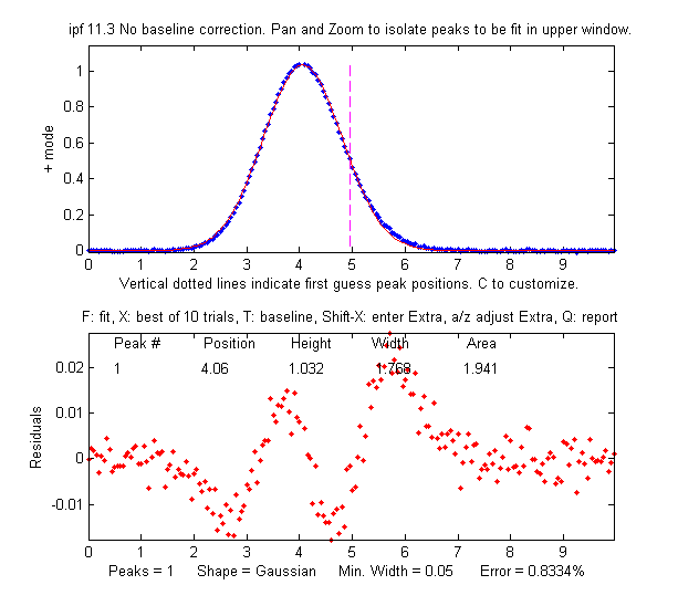
there more than one peak there? If we perform an unconstrained
iterative fit of a single Gaussian to the data, as shown in the figure on the
right, it shows little or no evidence of a second peak - the
residuals look pretty random. (If you could reduce the noise, or
ensemble-average even as few as 10
repeat signals, then the noise would be low enough to see
graphical evidence of a second peak). But as
it is, there is nothing that suggests a second peak.
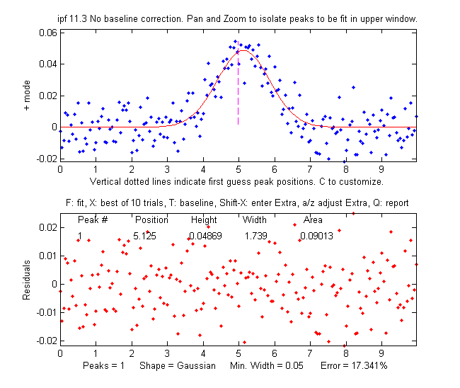
But suppose we suspect that there should
be another peak of the same Gaussian
shape just on the right side of the 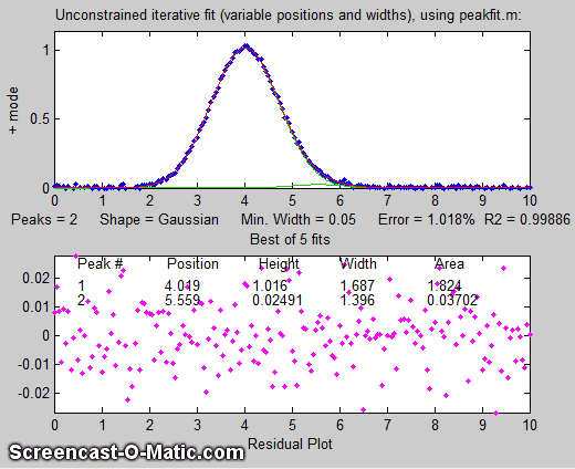 larger peak. We can try
fitting a pair of Gaussians to the data (figure on the left), but in
this case the random noise is enough that the fit is not stable.
When you run SmallPeak.m,
the script performs 20 repeat fits (NumSignals in line 20) with
the same underlying peaks but with 20 different random noise
samples, revealing the stability (or instability) of each
measurement method. The fitted peaks in Figure window 1 bounce
around all over the place as the script runs, as you can see in
the animation on the left. The fitting error is on average lower that the
single-Gaussian fit, but that by itself does not mean that the
peak parameters so measured will be reliable; it could just be
"fitting the noise". If it were
isolated all by itself, the small
peak would have a S/N ratio of about 5 and it could
be measured to a peak height precision of about 3%, but the
presence of the larger interfering peak makes the measurement
much more difficult. (Hint: After running SmallPeak.m the first
time, spread out all the figure windows so they can all be seen
separately and don't overlap. That way you can compared the
stability of the different methods more easily.)
larger peak. We can try
fitting a pair of Gaussians to the data (figure on the left), but in
this case the random noise is enough that the fit is not stable.
When you run SmallPeak.m,
the script performs 20 repeat fits (NumSignals in line 20) with
the same underlying peaks but with 20 different random noise
samples, revealing the stability (or instability) of each
measurement method. The fitted peaks in Figure window 1 bounce
around all over the place as the script runs, as you can see in
the animation on the left. The fitting error is on average lower that the
single-Gaussian fit, but that by itself does not mean that the
peak parameters so measured will be reliable; it could just be
"fitting the noise". If it were
isolated all by itself, the small
peak would have a S/N ratio of about 5 and it could
be measured to a peak height precision of about 3%, but the
presence of the larger interfering peak makes the measurement
much more difficult. (Hint: After running SmallPeak.m the first
time, spread out all the figure windows so they can all be seen
separately and don't overlap. That way you can compared the
stability of the different methods more easily.)

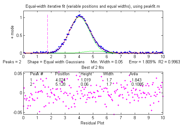
But suppose that we have reason to expect that the two peaks will have the same width, but we don't know what that width might be. We could
try an equal width Gaussian fit (peak shape #6, shown in Matlab/Octave
Figure window 2); the resulting fit is much more stable and
shows that a small peak is located at about x=5 on the right of
the bigger peak, shown below on the left. On the other
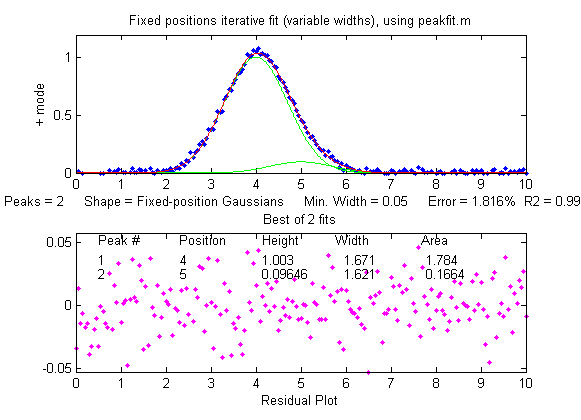
hand, if we know the peak positions beforehand, but not the widths, we can use a fixed-position Gaussian
fit (shape #16) shown on the right (Figure window 3). In
the very common situation where the objective is to measure an unknown
concentration of a known component,
then it's possible to prepare standard samples where the
concentration of the sought component is high enough for its
position or width to be determined with certainty.
So far all of these examples have used iterative
peak fitting with at least one peak parameter (position and/or
width) unknown and 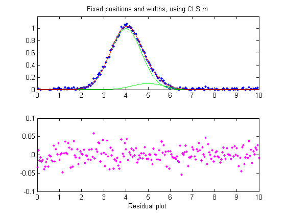 determined
by measurement. If, on the other hand, all
the peak parameters are known except the peak height,
then the faster and more direct classical least-squares regression
(CLS) can be employed (Figure window 4). In this case you need
to know the peak position and width of both the measured and the
larger interfering peaks (the computer will calculate their
heights). If the positions and the heights really are constant
and known, then this method gives the best stability and
precision of measurement. It's also computationally faster,
which might be important if you have lots of data to process
automatically.
determined
by measurement. If, on the other hand, all
the peak parameters are known except the peak height,
then the faster and more direct classical least-squares regression
(CLS) can be employed (Figure window 4). In this case you need
to know the peak position and width of both the measured and the
larger interfering peaks (the computer will calculate their
heights). If the positions and the heights really are constant
and known, then this method gives the best stability and
precision of measurement. It's also computationally faster,
which might be important if you have lots of data to process
automatically.
The problem with CLS is that it fails to give accurate
measurements if the peak position and/or width changes without
warning, whereas two of the iterative methods (unconstrained
Gaussian and equal-width Gaussian fits) can adapt to such
changes. It some experiments it quite common to have small
unexpected shifts in the peak position, especially in
chromatography or other flow-based measurements, caused by
unexpected changes in temperature, pressure, flow rate or other
instrumental factors. In SmallPeaks.m, such x-axis shifts can be
simulated using the variable "xshift" in line 18. It's initially
zero, but if you set it to something greater (e.g. 0.2) you'll
find that the equal-width Gaussian fit (Figure window 2) works
better because it can keep up with the changes in x-axis shifts.
But with a greater x-axis shift (xshift=1.0) even the equal-width fit has trouble. Still, if we know the separation between the two peaks, it's possible to use the findpeaksG function to search for and locate the larger peak and to calculate the position of the smaller one. Then the CLS method, with the peak positions so determined for each separate signal, shown in Figure window 5 and labeled "findpeaksP" in the table below, works better. Alternatively, another way to use the findpeaks results is a variation of the equal-width iterative fitting method in which the first guess peak positions (line 82) are derived from the findpeaks results, shown in Figure window 6 and labeled "findpeaksP2" in the table below; that method does not depend on accurate knowledge of the peak widths, only their equality.
Each time you run
SmallPeaks.m, all of these methods are
computed "NumSignals" times (set in
line 20) and compared in a table giving the average peak height
accuracy of all the repeat runs:
xshift=0
Unconstr. EqualW FixedP FixedP&W findpeaksP
findpeaksP2
35.607 16.849 5.1375
4.4437 13.384 16.849
xshift=1
Unconstr. EqualW FixedP FixedP&W findpeaksP
findpeaksP2
31.263 44.107 22.794
46.18 10.607 10.808
Bottom line. The more
you know about your signals, the better you can measure them. A
stable signal with known peak positions and widths is the most precisely
measurable in the presence of random noise ("FixedP&W"), but
if the positions or widths vary from measurement to measurement,
different methods must be used, and precision is degraded
because more of the available information is used to account for
changes other than the ones you want to measure.
This page is part of "A Pragmatic Introduction to Signal
Processing", created and maintained by Prof. Tom O'Haver ,
Department of Chemistry and Biochemistry, The University of
Maryland at College Park. Comments, suggestions and questions
should be directed to Prof. O'Haver at toh@umd.edu. Updated July, 2022.