This is
a simulation of several techniques described in this paper to
the quantitative measurement of a peak that is buried in excess of random noise, where the signal-to-noise (S/N) ratio is below 2. (Ordinarily, a
S/N ratio of 3 is desired for reliable detection).
The Matlab/Octave script LowSNRdemo.m performs the
simulations and calculations and compares the results
graphically, focusing on the behavior of each method as the S/N
ratio approaches zero. Four methods are compared:
(1) smoothing, followed by the peak-to-peak measure of the smoothed signal and background;
(2) a peak finding method based on the findpeakG function;
(3) unconstrained iterative least-squares fitting (INLS) based on the peakfit.m function; and
(4) constrained classical least squares fitting (CLS) based on the cls2.m function.
The
measurements
are carried out over a range of peak heights for which the S/N
ratio varies from 0 to 2. The noise
is random, constant, and white. Each time you run the
script, you get the same set of underlying signals but
independent samples of the random noise.
Results for the initial values in the script are shown
in the plots on the left and in the table printed below, both of
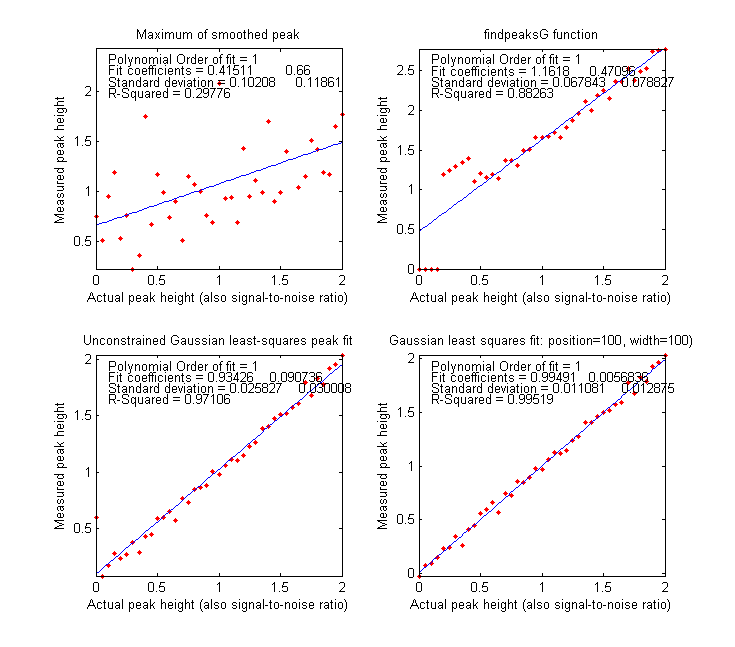
which are created by the script LowSNRdemo.m. The graphs on the
left show correlation plots of the measured peak height vs the
real peak height, which should ideally be a straight line with a
slope of 1, an intercept of zero, and an R-squared of 1.
As you can see, the simplest smoothed-peak method (upper left)
is completely inadequate, with a low slope (because smoothing
reduces peak height) and a high intercept (because even smoothed
noise has a non-zero peak-to-peak value). The findpeaks function
(upper right) works OK for height for higher peak heights but
fails completely below a S/N ratio of 0.5 because the peak
height falls below the amplitude threshold setting. In
comparison, the two least-squares techniques work much better,
reporting much better values of slope, intercept of zero, and
R-squared. But if you look closely at the low end of the peak
height range, near zero, you can see that the values reported by
the unconstrained fit (lower left) occasionally stray from the
line, whereas the constrained fit (lower right) decrease
gracefully all the way to zero every time you run the script.
Essentially the reason why it's even possible to make
measurements at such low S/N ratios is that the data density is very high: that is, there are many data points in each signal
(about 1000 points across the half-width of the peak with the
initial script values).
The results are summarized in the table below. The height errors are reported as a percentage of the maximum height (initially 2). (For the first three methods, the peak position is also measured and its relative accuracy is reported. The constrained classical least squares fitting does not measure peak position but rather assumes that it remains fixed at the initial value of 100). You can see that the CLS method has a slight edge in accuracy, but you have to consider also that this method works well only if the peak shape, position, and width are known. The unconstrained iterative method can track changes in peak position and width.

Number of points in half-width of
peak: 1000
Method
Height
Error Position Error
Smoothed peak
21.2359% 120.688%
findpeaksG.m
32.3709% 33.363%
peakfit.m
2.7542%
4.6466%
cls2.m
1.6565%
You can change
several of the factors in this simulation to test the robustness
of these methods. Search for the word 'change' in the comments
for values that can be changed. Reduce MaxPeakHeight (line 8) to
make the problem harder. Change peak position and./or width
(lines 9 and 10) to show how the CLS method fails. As usual, the
more you know, the better your results. Change the increment
(line 4) to change the data density; more data is always better.
(Surprisingly, as it will be shown in Appendix
U: Measurement Calibration, it
is not even necessary to have an accurate peak shape model
in order to get a good correlation between measured
and actual height).
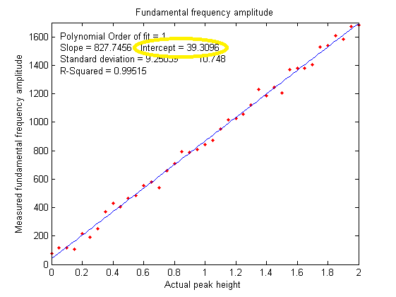
LowSNRdemo.m also computes the power spectrum of the signal and
the amplitude (square root of the power) of the fundamental,
where most of the power of a broad Gaussian peak falls, and
plots it in Figure(2). The correlation to peak
height is similar to the CLS method, but the
intercept is higher because there
is a non-zero quantity of noise even in that one frequency slice
of the power spectrum.
We are now, in the 21st century, into the era of "big
data", where high-speed automated data systems can acquire,
store, and process greater quantities of data than ever before.
As this little example shows, greater quantities of data allow
researchers to probe deeper and measure smaller effects that
previously.
This page is part of "A Pragmatic Introduction to Signal
Processing", created and maintained by Tom O'Haver, Professor
Emeritus, Department of Chemistry and Biochemistry, The University
of Maryland at College Park. Comments, suggestions and questions
should be directed to Prof. O'Haver at toh@umd.edu. Updated July, 2022.