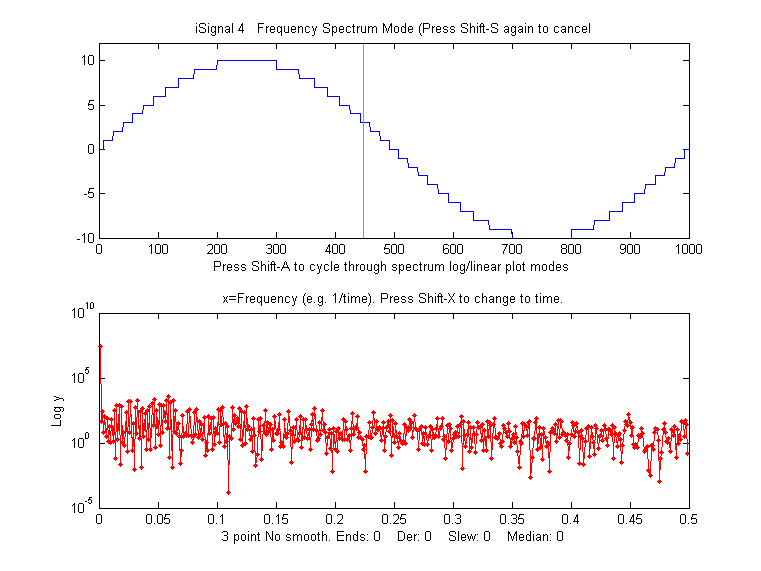
Digitization noise, also called quantization noise, is an artifact caused by the rounding or truncation of numbers to a fixed number of figures. It can originate in the analog-to-digital converter that converts an analog signal to a digital one, or in the circuitry or software involved in transmitting the digital signal to a computer, or even in the process of transferring the data from one program to another, as in copying and pasting data to and from a spreadsheet. The result is a series of non-random steps of equal height. The frequency distribution is white, because of the sharpness of the steps, as you can see by observing the power spectrum.
The
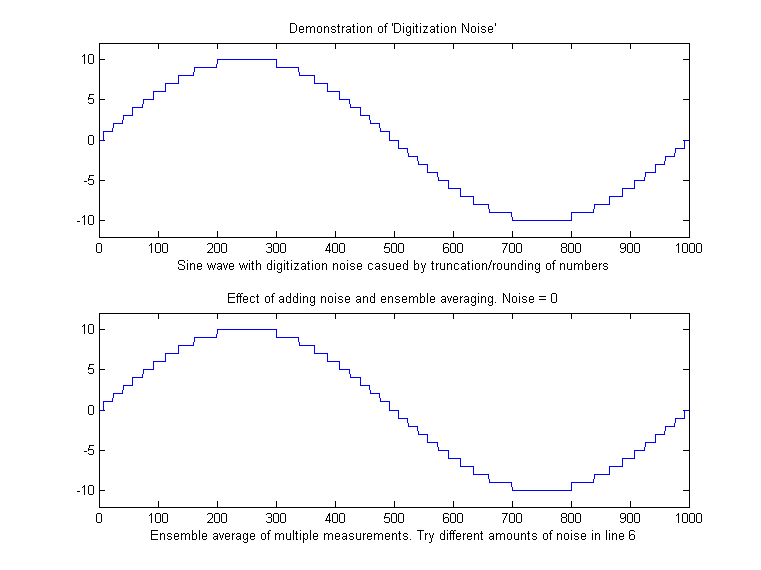
figure on the left, top panel, shows the effect of integer
digitization on a sine wave with an amplitude of +/- 10.
Ensemble averaging, which is usually the most effective of
noise reduction techniques, does not reduce this type of noise
(bottom panel) because it is non-random.
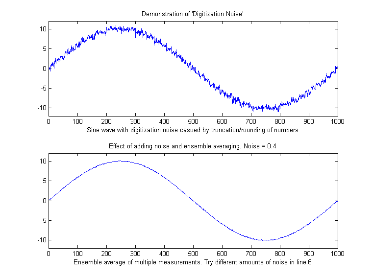
 Interestingly,
if additional random noise is present in the signal, then
ensemble averaging becomes effective in reducing both the random noise and the digitization
noise. In essence, the added noise randomizes the
digitization, allowing it to be reduced by ensemble averaging.
Moreover, if there is insufficient random noise already in the
signal, it can be beneficial to add additional noise
artificially! The script RoundingError.m illustrates this
effect, as shown the animation on the right, which shows the
digitized sine wave with gradually increasing amounts of added
random noise in line 8 (generated by the
randn.m function) followed by ensemble averaging of 100
repeats
(in lines 17-20). Look closely at the
waveform in this animation as it changes in response to the
random noise addition shown in the title. You can clearly see
how the noise starts out mostly quantization noise but then
quickly decreases as small but increasing amounts of random
noise are added before the ensemble averaging step, then
eventually increases as too much noise is added. The optimum
standard deviation of random noise is about 0.36 times the
quantization size, as you can demonstrate by adding lesser or
greater amounts via the variable Noise in line 6 of this
script. Note that this works only for ensemble averaged
signals where the noise is added before the quantification.
Interestingly,
if additional random noise is present in the signal, then
ensemble averaging becomes effective in reducing both the random noise and the digitization
noise. In essence, the added noise randomizes the
digitization, allowing it to be reduced by ensemble averaging.
Moreover, if there is insufficient random noise already in the
signal, it can be beneficial to add additional noise
artificially! The script RoundingError.m illustrates this
effect, as shown the animation on the right, which shows the
digitized sine wave with gradually increasing amounts of added
random noise in line 8 (generated by the
randn.m function) followed by ensemble averaging of 100
repeats
(in lines 17-20). Look closely at the
waveform in this animation as it changes in response to the
random noise addition shown in the title. You can clearly see
how the noise starts out mostly quantization noise but then
quickly decreases as small but increasing amounts of random
noise are added before the ensemble averaging step, then
eventually increases as too much noise is added. The optimum
standard deviation of random noise is about 0.36 times the
quantization size, as you can demonstrate by adding lesser or
greater amounts via the variable Noise in line 6 of this
script. Note that this works only for ensemble averaged
signals where the noise is added before the quantification.
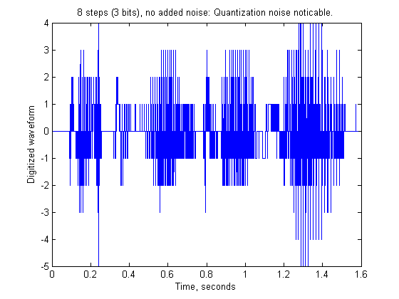 An audible example of this
idea is illustrated by the Matlab/Octave script DigitizedSpeech.m,
which starts with an audio recording of the spoken phrase
"Testing, one, two, three", previously recorded at 44000 Hz
and saved in WAV format (TestingOneTwoThree.wav) and in
.mat format (testing123.mat),
rounds off the amplitude data progressively to 8 bits (256
steps; sound link),
shown on the left, 4 bits (16 steps; sound link), and 1 bit (2 steps;
sound link), and
then the 2-step case again with random
white noise added before the rounding (2 steps + noise; sound link), plots the waveforms
and plays the resulting sounds, demonstrating both the
degrading effect of rounding and the remarkable improvement
caused by adding noise. (Click on these sound links to hear
the sounds on your computer). Although the computer program in this
case does not perform an explicit ensemble averaging operation as does RoundingError.m,
it's likely that the neurons of the hearing center of your
brain provide that function by virtue of their response time
and memory effect.
An audible example of this
idea is illustrated by the Matlab/Octave script DigitizedSpeech.m,
which starts with an audio recording of the spoken phrase
"Testing, one, two, three", previously recorded at 44000 Hz
and saved in WAV format (TestingOneTwoThree.wav) and in
.mat format (testing123.mat),
rounds off the amplitude data progressively to 8 bits (256
steps; sound link),
shown on the left, 4 bits (16 steps; sound link), and 1 bit (2 steps;
sound link), and
then the 2-step case again with random
white noise added before the rounding (2 steps + noise; sound link), plots the waveforms
and plays the resulting sounds, demonstrating both the
degrading effect of rounding and the remarkable improvement
caused by adding noise. (Click on these sound links to hear
the sounds on your computer). Although the computer program in this
case does not perform an explicit ensemble averaging operation as does RoundingError.m,
it's likely that the neurons of the hearing center of your
brain provide that function by virtue of their response time
and memory effect.
This page is part of "A Pragmatic Introduction to Signal
Processing", created and maintained by Prof. Tom O'Haver ,
Department of Chemistry and Biochemistry, The University of
Maryland at College Park. Comments, suggestions and questions
should be directed to Prof. O'Haver at toh@umd.edu. Updated July, 2022.