This section contains detailed descriptions of the MathViews functions. Each function description contains a synopsis of the calling sequence, a description of how the function operates, an example of usage, and a list of related functions.
Synopsis:
abs(expr)
Description:
The abs function computes the absolute value of its argument.
If the argument is an array, the function operates on each element of the array. The result is an array with the same dimensions as the argument. If the argument has complex elements, the complex modulus:
![]()
is used to compute the result.
If the argument is a text string, the function converts the text string into its integer equivalent.
Example:
|
INPUT |
OUTPUT |
| a = -5 |
abs(a)
ans = 5 |
| A =
1 -2 -3 3 -1 -3 |
abs(A)
ans = 1 2 3 3 1 3 |
| t = 'MathViews' |
abs(t)
ans = 77 97 116 104 86 105 101 119 115 |
| z = 2 + 3j |
abs(z)
ans = 3.6056 |
Related Topics:
Synopsis:
acos(expr)
Description:
The acos function computes the arccosine (inverse cosine) of its argument, returning a value in radians.
If the argument is a real scalar and the absolute value of the argument is 1.0, the result is a real scalar in the range of [0,]. If the absolute value of the argument is 1.0, the result is a complex scalar.
If the argument is an array, the function operates on each element of the array. The result is an array with the same dimensions as the argument.
If the argument has complex element(s), the complex arccosine:
![]()
is used to compute the result.
Example:
|
INPUT |
OUTPUT |
| A =
1 -2 3 -1 |
acos(A)
ans = 0 3.1416 - 1.317 j 1.7627 j 3.1416 |
| z = 2 + 3 j |
acos(z)
ans = 1.0001 - 1.9834 j |
Related Topics:
cos, cosh, sin, exp, log, log10
Synopsis:
acosh(expr)
Description:
The acosh function computes the hyperbolic inverse cosine of its argument.
Example:
|
INPUT |
OUTPUT |
| acosh([0:0.5:2]) |
ans =
0 + 1.571 j 0 + 1.047 j 0 0.9624 1.317 |
| x=1:0.2:10;
plot(x,acosh(x)),grid |

|
Related Topics:
Synopsis:
all(expr)
Description:
The all function tests whether all the elements of its argument are 1.
If the argument is a vector, then the function returns a 1, providing that all the elements of the argument are nonzero; otherwise a 0 is returned.
If the argument is a matrix, the function operates on each column. The function returns a row vector with elements in the set {0,1} pertaining to the condition of the columns.
Example:
|
INPUT |
OUTPUT |
| x = 1 2 3 4 |
all(x)
ans = 1 |
| y = 1 2 3 0 |
all(x)
ans = 1 |
| A =
1 -2 3 3 -1 0 |
all(A)
ans = 1 1 0 |
Related Topics:
Synopsis:
angle(expr)
Description:
The angle function computes the phase of its argument in radians.
If the argument is an array, the function operates on each element of the array. The result is an array with the same dimensions as the argument.
This function is meaningful for complex arguments as well as real arguments, and it returns a real value in either case.
The phase of real numbers is 0.
Example:
|
INPUT |
OUTPUT |
| z = 3 + 5i |
angle(z)
ans = 1.03038 |
| A = [z,z;z,z] |
angle(A)
ans = 1.03038 1.03038 1.03038 1.03038 |
Related Topics:
Synopsis:
any(expr)
Description:
The any function tests whether any of the elements of its argument is a 1.
If the argument is a vector, the function returns 1, providing that any of the elements of the argument are nonzero; otherwise a 0 is returned.
If the argument is a matrix, the function operates on each column. The function returns a row vector with elements in the set {0,1} pertaining to the condition of the columns.
Example:
|
INPUT |
OUTPUT |
| x = 1 2 3 4 |
any(x)
ans = 1 |
| y = 1 2 3 0 |
any(x)
ans = 1 |
| A =
1 -2 0 3 -1 0 |
any(A)
ans = 1 1 0 |
Related Topics:
Synopsis:
asin(expr)
Description:
The asin function computes the arcsine (inverse sine) of its argument, returning a value in radians.
If the argument is a real scalar and the absolute value of the argument is 1.0, then the result is a real scalar in the range [/2,/2]. If the absolute value of the argument is 1.0, then the result is a complex scalar.
If the argument is an array, the function operates on each element of the array. The result is an array with the same dimensions as the argument.
If the argument has complex element(s), the complex arcsine:
![]()
is used to compute the result.
Example:
|
INPUT |
OUTPUT |
| A =
1 -2 3 -1 |
asin(A)
ans = 1.5708 -1.571 + 1.317 j 1.5708 - 1.7627 -1.571 |
| z = 2 + 3 j |
asin(z)
ans = 0.5707 + 1.9834 j |
Related Topics:
Synopsis:
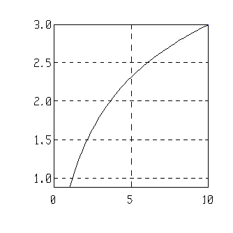
asinh(expr)
Description:
The asinh function computes the hyperbolic inverse sine of its argument.
Example:
|
INPUT |
OUTPUT |
| asinh([0:0.5:2]) |
ans =
0 0.4812 0.8814 1.195 1.444 |
| x=1:0.2:10;
plot(x,asinh(x)),grid |
|
Related Topics:
Synopsis:
atan(expr)
Description:
The atan function computes the arctangent (inverse tangent) of its argument, returning a value in radians.
If the argument is a real scalar, the result is a real scalar in the range [/2,/2].
If the argument is an array, the function operates on each element of the array. The result is an array with the same dimensions as the argument.
If the argument has complex element(s), the complex arctangent:
![]()
is used to compute the result.
Example:
|
INPUT |
OUTPUT |
| A =
1 -2 3 -1 |
atan(A)
ans = 0.7854 -1.107 1.249 -0.7854 |
| z = 2 + 3 j |
atan(z)
ans = 1.4099 + 0.2291 j |
Related Topics:
atan2, tan, sin, cos, exp, log
Synopsis:
atan2(expr1,expr2)
Description:
The atan2 function computes the 4th quadrant arc tangent of expr1 ./ expr2, returning a value in radians.
If the argument is a real scalar, the result is in the range [-,+].
If the arguments are two arrays, the function operates on each element of the corresponding arrays:
![]() .
.
If the argument has complex element(s), the imaginary parts of the complex element(s) is(are) ignored during the computation. Only the real parts are used in the computation.
Example:
|
INPUT |
OUTPUT |
| x = 1 2 3 4
y = 2 4 6 8 |
atan2(x,y)
ans = 0.4636 0.4636 0.4636 0.4636 |
| xc = x + 5i
yc = y + 4j |
atan2(xc,yc)
ans = 0.4636 0.4636 0.4636 0.4636 |
Notice that although both xc and yc are complex vectors, the atan2 function ignores the imaginary parts when computing the arc tangent.
Synopsis:
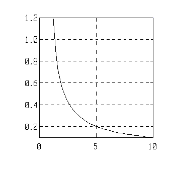
atanh(expr)
Description:
The atanh function computes the hyperbolic inverse tangent of its argument.
Example:
|
INPUT |
OUTPUT |
| atanh([0 0.5 1.5 2]) |
ans =
0 0.5493 0.8047 + 1.571 j 0.5493 + 1.571 j |
| x=1.2:0.2:10;
plot(x,atanh(x)),grid |
|
Related Topics:
Synopsis:
axis
axis([xmin, xmax, ymin, ymax])
axis('format') ; format can be either square or normal.
Description:
The axis function is used to manually scale the x-y range of a plot.
If axis is called with no argument, it freezes the current displayed plot's dimension for subsequent plots until it is reset or reassigned. The function returns the previous dimensions before the update. Executing the axis function again without an argument resets the plotting procedure to auto-scaling.
If axis is called with an argument, the argument must be a four element vector, consisting of [xmin, xmax, ymin, ymax]. Axis will manually scale the plot to those dimensions, returning the dimensions of the update. To resume auto-scaling, execute the axis function without an argument.
The format string is used to control the aspect ratio of the graphics images. The parameter normal is used to tell MathViews to use the current display device's aspect ratio. The parameter square is used to tell MathViews to auto-adjust to a square aspect ratio. Using the format functions keeps the current state of the axis; i.e. if the current state is auto-scaling, then executing axis('square') keeps the state auto-scaling.
Example:
|
INPUT |
OUTPUT |
| axis |
ans =
0 1 0 1 |
| axis('normal') |
Axis Fixed (current state)
axis('normal') ans = 1 10 0.01991 0.9788 |
| axis([ 0 10 0 10]) |
ans =
0 10 0 10 |
Related Topics:
Synopsis:
balance(expr)
[T, B] = balance(expr)
Description:
The balance function attempts to improve the conditioning of a matrix.
The argument must be a square matrix. The function attempts to find a similarity transformation T, a diagonal matrix, such that T makes the row and column norms approximately equal. Hence the balanced matrix is inv(T)*expr*T.
When two return arguments are specified, then T is the diagonal transformation matrix, and B is the balanced matrix inv(T)*expr*T.
This function is meaningful for complex arguments as well as real arguments, and it returns a real value in either case.
Example:
|
INPUT |
OUTPUT |
| a=[4 1;8 -4]
[T,A]=balance(a) |
[T,A]=balance(a) T = 0.5 0 0 1 A = 4 2 4 -4 |
| T\a*T % =A |
ans =
4 2 4 -4 |
Related Topics:
Synopsis:
blackman(N)
Description:
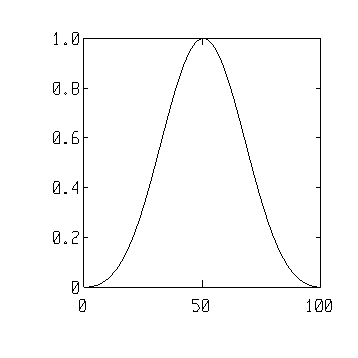
The blackman function creates an N-point Blackman window in a column vector.
The Blackman window function is used to reduce leakage in the output of a fast Fourier transform (FFT) to a greater degree than would be obtained from using a rectangular window function.
Leakage is due to the difficulty of capturing exactly one period, or exactly some multiple of periods, of the signal being processed. If the window is rectangular, the resulting truncation causes a great deal of leakage. Leakage can be reduced by using certain nonrectangular window functions, with specific characteristics. Importantly:
1) Side lobes in the Fourier transform of the window function must be significantly smaller than the side lobes in the Fourier transform of a rectangular function.
2) The main lobe of the window-function Fourier transform must be narrow enough to prevent important signal information from being lost.
The Blackman window function possesses these characteristics, as do the Hamming and Hanning window functions, which are also available with MathViews.
These characteristics are necessary because, due to sampling and the accompanying truncation, energy in a DFT output appears at a series of specific frequencies. If fs is the sampling frequency and N is the number of samples, the specific frequencies range from 0 Hz to fs/2 Hz, and they are equally spaced fs/N Hz apart. As long as N contains one period, or multiple periods, of the signal, then all of the series of specific frequencies of the DFT output can pass. If N does not contain one or a multiple of periods, at least one of the series is blocked and its/their energy is distributed to the other components of the spectrum.
(next page)
Example:
|
INPUT |
OUTPUT |
| blackman(5)' |
ans =
0 0.34 1 0.34 0 |
| plot(blackman(100)) |
|
Related Topics:
wmerit, hamming, hanning, wbartlet, wrect, wsina
Synopsis:
casesen
casesen [on/off]
Description:
The function casesen is used to toggle case sensitivity in Mathviews.
Mathviews is always initialized to case sensitive inputs during startup, i.e. Mathviews will distinguish between lowercase and uppercase variables. The command can be used by itself to toggle the case sensitivity state. The command can also be used with the keywords [on/off] to explicitly specify the mode.
Example:
|
INPUT |
OUTPUT |
| casesen on
aa = 1 AA = 9 aa AA |
aa =
1 AA = 9 aa ans = 1 AA ans = 9 |
| casesen off
aa AA |
%starting here, case sensitivity is off aa ans = 1 AA ans = 1 |
| casesen on
aa AA |
%starting here, case sensitivity is on
aa ans = 1 AA ans = 9 |
Synopsis:
ceil(expr)
Description:
The ceil function rounds the element(s) of its argument to the nearest integer towards .
The argument can be a scalar, a vector, or a matrix.
If the argument has complex element(s), the function operates on both the real and the imaginary parts of the element(s).
Example:
|
INPUT |
OUTPUT |
| A =
-0.3 5.6 4.5 -0.02 5.1 5.6 |
ceil(A)
ans = 0 6 5 0 6 6 |
| z = 2.3 + 4.5j |
ceil(z)
ans = 3 + 5j |
Related Topics:
Synopsis:
chdir (directory)
Description:
The chdir command makes the named directory the current working directory. It also modifies the , _MVPWD variable to reflect the new working directory.
NOTE: The search path for m-files always includes the current working directory. Changing the working directory can change availability of script files and functions.
Example:
chdir docs Changes the current working directory to the directory, docs.
Related Topics:
dir, type, delete, who, whos, _MVPWD
Synopsis:
C = chol(A)
Description:
The chol function computes the Cholesky factorization of its argument, a non-singular symmetric matrix, A, and produces a lower triangular matrix, C, as the result.
The upper triangular matrix is the transpose of C. Thus A = C * C', which is known as the Cholesky factorization of A. A must be positive definite (see positive definite discussion in linear algebra books).
Example:
|
INPUT |
OUTPUT |
| A=[1 4 2 3;4 6 2 9;2 2 7 8;3 9 8 9]
B=A'*A C=chol(B) C*C' |
C=chol(B)
C = 5.477 0 0 0 10.77 4.579 0 0 8.764 2.533 6.147 0 14.97 0.3785 3.228 0.5514 |
| C=chol(A) % generates error |
Error: A is not positive definite. |
Related Topics:
Synopsis:
cla
Description:
The cla command clears the Output window
Example:
|
cla |
|
| Clears the output window. |
Related Topics:
Synopsis:
clc
Description:
The clc function clears text from the Output window.
Text can also be moved out of the output window using the scroll arrows.
Example:
clc
Related Topics:
Synopsis:
clear
clear functions
clear variable1 variable2 ...
Description:
The clear function clears variables from MathViews' memory.
Executing the command with no argument(s), will clear all variables and functions currently in memory. Executing the command with multiple arguments will clear those arguments. Multiple arguments must be separated by at least a single space. The command also clears functions residing in memory.
Upon completing execution of the clear function, MathViews will execute the commands contained in the file restart.m. This allows the environment to be reset to a default starting condition.
Example:
clear
clear x1, x2
clear median
Related Topics:
Synopsis:
clock
Description:
The clock function computes the current date and time in a six elements row vector.
The clock vector has the format [year month day hour minute fraction_of_seconds].
Example:
|
INPUT |
OUTPUT |
| t1=clock
z=eye(50); t2=clock etime(t2,t1) |
t1=clock
t1 = 93 1 15 11 0 36.1 t2=clock t2 = 93 1 15 11 0 39.0 etime(t2,t1) ans = 3.1 |
Related Topics:
Synopsis:
cntrlb(data)
Description:
The cntrlb function generates a contour line plot in the same manner as the contour function. In addition, the cntrlb function also plots the contour level numbers.
Example:
|
INPUT |
OUTPUT |
| n=8;
x=(0:n)/n; y=x.*(1.2-x); y /= max(y); z=y'*y; cntrlb(z) |

|
Related Topics:
Synopsis:
compan(expr)
Description:
The compan function computes the companion matrix.
The companion matrix is a square matrix, whose first row is expr(2:n)/expr(1).
Example:
Consider solving the roots for equation: ![]()
|
INPUT |
OUTPUT |
| p := [1 -3 -3 7 6]
eig(compan(p)) |
ans = 3 2 -1 + 6.294e-09 j -1 - 6.294e-09 j |
| angle(ans) |
ans =
0 0 3.142 -3.142 |
Related Topics:
Synopsis:
computer - Operating system
Description:
The computer function is a compatibility function. It returns the string 'WIN', indicating that MathViews is runing in the Microsoft Windows environment.
Example:
|
INPUT |
OUTPUT |
| computer |
computer
ans = WIN |
Related Topics:
none
Synopsis:
cond(A)
Description:
The cond function computes the condition number of matrix A.
The condition number indicates the sensitivity of matrix A to error when solving the problem of the form Ax = b. A must be a square matrix and non-singular. A high condition number is error prone when doing matrix inversions or solving systems of linear equations. The condition number is computed by the ratio of the max and min value of the singular value decomposition of A.
The condition number is computed using the 2-norm.
Example:
|
INPUT |
OUTPUT |
| A =
1 1 2 2 4 -3 3 6 -5 |
cond(A)
ans = 243.226 |
| norm(A)*norm(inv(A))
ans = 243.226 |
Note: the condition number is also defined to be norm(A)*norm(inv(A)). Also, this is a well behaved matrix. The condition number is relatively small as compared to the reciprocal of the machine epsilon.
Related Topics:
Synopsis:
conj(expr)
Description:
The conj function computes the complex conjugate of its argument.
If the argument is a complex scalar, the result is the complex conjugate of the argument. Real scalars are left unchanged.
If the argument is an array, the function operates on each element of the array, and the result is an array with the same dimensions as the argument.
Example:
|
INPUT |
OUTPUT |
| z = 4 - 5 j
conj(z) |
ans = 4 + 5 j |
| expr =
7 5 + 6 j 4 - 2 j -3 - 1 j conj(expr) |
ans = 7 5 - 6 j 4 + 2 j -3 + 1 j |
Related Topics:
Synopsis:
contour(data)
contour(data, [vc,lv])
contour(data, [vc,lv], xrange vector, yrange vector)
Description:
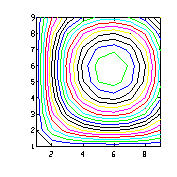
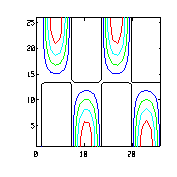
The contour function generates a contour lines plot.
The argument, data, is an array (matrix) containing the data to generate the contour plot. The data argument must be a real 2-dimensional array, i.e. a square matrix.
If the integer value, lv, is included, then the contour plot will include up to lv contour levels. If the vector argument, vc, is included instead of the argument lv, then the contour plot will include only levels specified by the elements of the vc vector.
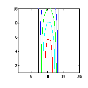
Also, when specifying the xrange and yrange vectors, their elements must contain values where the contour is to be plotted. For sample, [0 10] will only show contour points at 0 and 10. However, [1:10] will show contour points at 1 through 10.
Example:
|
INPUT |
OUTPUT |
| n=8;
x=(0:n)/n; y=x.*(1.2-x); y /= max(y); z=y'*y; contour(z) |
|
| x = 0:.5:4*pi;
y = 0:.5:4*pi; [XX,YY]=meshdom(x,y); ZZ = 0.5*sin(XX).*cos(YY./4); contour(ZZ, [ 0:.1:1]) |
|
| contour(ZZ,[0:.1:1],[1:20],[1:10]) |
|
Related Topics:
Synopsis:
c = conv(expr1, expr2)
Description:
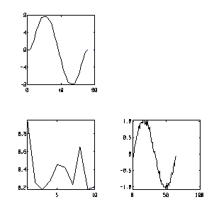
The conv function performs a convolution of the two vectors, expr1 and expr2. The convolution is expressed as:
![]()
where N is the length of the vectors expr1 and expr2.
Example:
|
INPUT |
OUTPUT |
| x=1:6
y=[1 1 1] z=conv(x,y) |
z =
1 3 6 9 12 15 11 6 |
| subplot(221)
n=64; plot(rand(1,10)) %noisy signal x=sinw(n)+(rand(1,n)-0.5)/4; % moving average y=ones(1,8) plot(x) plot(conv(x,y)) subplot(111) |
|
Related Topics:
Synopsis:
cos(expr)
Description:
The cos function computes the cosine of its argument.
If the argument is an array, the function operates on each element of the array. The result is an array with the same dimensions as the argument.
If the argument has complex element(s), then the complex cosine function:
![]()
is used to compute the result.
Example:
|
INPUT |
OUTPUT |
| z = 3 + 4j |
cos(z)
ans = -27.03 - 3.8512 j |
Related Topics:
Synopsis:
cosh(expr)
Description:
The cosh function computes the hyperbolic cosine of its argument.
If the argument is an array, the function operates on each element of the array. The result is an array with the same dimensions as the argument.
The cosh function is defined as:
![]() .
.
Example:
|
INPUT |
OUTPUT |
| z = 3 + 4j |
cosh(z)
ans = -6.58066 - 7.58155 j |
Related Topics:
Synopsis:
cosw( points, cycles, freq, phase)
Description:
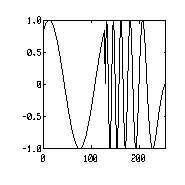
The cosw function is used to create sinusoidal waveforms.
The arguments are:
|
points |
number of elements of the waveform sequence |
| cycles |
the number of cycles of the waveform |
| freq |
the frequency deviation of the waveform |
| phase |
the initial phase of the waveform |
The cosw function is identical to the sinw function except that the default value of the initial phase is 90 degrees rather than 0.
Example:
|
INPUT |
OUTPUT |
| % half a cycle
plot(cosw(256,0.5)) |
|
| n=128
% two segments of 32 points np=[n n] % 2 cycles and 4 cycles f0=[1 10] % frequency sweep df=[0 -10] % initial phase ph0=[pi/3 0] plot(cosw(np,f0,df,ph0)) |
|
Related Topics:
Synopsis:
cov(A)
cov(a, b)
Description:
The cov function computes the covariance matrix of its argument.
Example:
|
INPUT |
OUTPUT |
| x=1:4
cov(x) |
x =
1 2 3 4 cov(x) ans = 1.25 |
| cov(x'*x) |
cov(x'*x)
ans = 1.25 2.5 3.75 5 2.5 5 7.5 10 3.75 7.5 11.25 15 5 10 15 20 |
Related Topics:
Synopsis:
cumprod(expr)
Description:
The cumprod function computes the cumulative product of its argument.
If the argument is a real scalar, the result is the same as the argument
If the argument is a vector, the result is the cumulative product of the argument's elements.
If the argument is a matrix, the function operates on each column. The function returns a row vector with elements being the cumulative product of each column of the matrix.
Example:
|
INPUT |
OUTPUT |
| a = 4 |
cumprod(a)
ans = 4 |
| A =
2 4 1 3 2 5 3 5 2 |
cumprod(A)
ans = 2 4 1 6 8 5 18 40 10 |
Related Topics:
Synopsis:
cumsum(expr)
Description:
The cumsum function computes the cumulative sum of its argument.
If the argument is a real scalar, the result is the same as the argument
If the argument is a vector, the result is the cumulative sum of the argument's elements.
If the argument is a matrix, the function operates on each column. The function returns a row vector with elements being the cumulative sum of each column of the matrix.
Examples:
|
INPUT |
OUTPUT |
| A = 3 5 7 |
cumsum(A)
ans = 3 8 15 |
| A =
2 4 1 3 2 5 3 5 2 |
cumsum(A)
ans = 2 4 1 5 6 6 8 11 8 |
Related Topics:
Synopsis:
delete (filename)
Description:
The delete command removes the named file from the current directory. Pathnames, wild cards and drive designators may be used.
Example:
delete temp.tmp Deletes the file, temp.tmp from the current directory.
Related Topics:
Synopsis:
det(expr)
Description:
The det function computes the determinant of its argument.
The argument must be a square matrix. The determinant of a complex matrix is also supported.
Example:
|
INPUT |
OUTPUT |
| B =
2 3 4 4 5 6 5 10 7 |
det(B)
ans = 16 |
| B =
2 3 + 3 j 4 4 5 6 + 4 j 5 10 + 6 j 7 |
det(B)
ans = 4 + 10 j |
Related Topics:
Synopsis:
dft(X)
Description:
The dft function computes the discrete Fourier transform of its argument. The discrete Fourier transform (DFT) is the discrete-time equivalent of the continuous-time Fourier transform. Given X(f) as the continuous Fourier transform of a coutinuous time signal x(t), then the DFT of the sampled time signal, x(n), is a sequence of samples of X(f), equally spaced in frequency. The DFT of a signal, x(n), is calculated as:
![]()
where
![]()
Example:
|
INPUT |
OUTPUT |
| dft(1:7)' |
dft(1:7)'
ans = 28 -3.5 - 7.268 j -3.5 - 2.791 j -3.5 - 0.7989 j -3.5 + 0.7989 j -3.5 + 2.791 j -3.5 + 7.268 j |
| x=[0 0 1 zeros(1,50)];
plot(imag(dft(x'))) |

|
Related Topics:
Synopsis:
diag(A)
diag(A, k)
Description:
The diag function returns the diagonal of its argument.
If the argument is a vector, the function is equivalent to diag(A, 0) and will return a diagonal matrix with the elements of A as diagonal elements. If k > 0, then the elements of the argument, will be the k-th diagonal above the main diagonal. If k < 0, the elements of the argument, will be the k-th diagonal below the main diagonal.
If the argument is a matrix, the function returns a column vector consisting of the diagonal elements of A. If k > 0, then a column vector consisting of the k-th diagonal elements above the main diagonal is returned.
Example:
|
INPUT |
OUTPUT |
| A =
1 2 3 4 2 3 5 5 3 10 5 6 4 9 6 7 |
diag(A)
ans = 1 3 5 7 |
| L =
1 1 0 0 |
diag(A(:,L))
ans = 1 3 |
| diag(A,-1)
ans = 2 10 6 |
Related Topics:
Synopsis:
diary
diary filename
diary [on/off]
Description:
The diary command generates a file, filename, containing all subsequent input commands and most outputs (except graphics) from MathViews' Interactive window and Output window.
If filename is not specified, then mathview.dry is generated. The diary function by itself toggles the diary mode. Diary can also be used with keywords [on/off] to explicitly specify the diary mode. MathViews is initialized to diary off during startup.
The name of the diary file cannot be 'on' or 'off'
Example:
|
INPUT |
| diary on
disp('MathViews') x = [ ] A = eye(3,3) diary off |
Related Topics:
Synopsis:
diff(expr)
diff(expr, n)
Description:
The diff function computes the approximate derivative.
The function operates following the rule:
x(i) = x(i+1) - x(i) for 1 <= i <= n,
where n is the number of elements in a vector.
If the argument is a vector with n elements, the function returns a vector representing its difference with n-1 number of elements.
If the argument is a matrix, the function operates on each column of the matrix.
Example:
|
INPUT |
OUTPUT |
| x =
1 2 3 4 5 6 7 8 9 4 7 5 0 6 2 1 |
diff(x)
ans = 8 2 4 1 -5 0 -5 -7 |
| diff(x',2)'
ans = 0 0 0 0 0 0 8 -5 -3 11 -10 3 |
Related Topics:
Synopsis:
dir
dir(</option> <directory>)
Description:
The command dir returns a list of the files in a directory. It is a generic file manipulation command that is analogous to its MS DOS counterpart, dir. Pathnames, wildcards, /p and /w options, and drive designators can be used. If no directory pathname is specified, dir returns a list of the files in the current directory.
Examples:
dir d* Lists all the of the subdirectories and files in the current directory that begin with the letter, D. dir/p A: Lists al of the directories and files in the home directory of the A drive.
Related Topics:
chdir, delete, type, who, whos
Synopsis:
disp(expr)
Description:
The disp function displays the contents of its argument.
If the argument is a text string, the string is displayed in the output window.
If the argument is a variable, the content(s) of the argument is(are) displayed in the output window without displaying the name of the variable.
Example:
|
INPUT |
OUTPUT |
| t = 'MathViews' |
disp(t)
mathviews |
| A =
2 4 1 3 2 5 3 5 2 |
disp(A)
2 4 1 3 2 5 3 5 2 |
Related Topics:
Synopsis:
echo
echo [on/off] [all]
echo function [on/off]
Description:
The echo command tells MathViews to display the statements of an M-file as it executes.
The effect of the echo command depends on whether the M-file currently being executed is a script file or a function file.
With script files, the command toggles the echo [on/off] mode for any currently running script M-file. When the echo mode is on, script M-file statements are displayed before execution. Echo [on/off] explicitly specifies the echo mode.
With function files, when echo is enabled, the function file is interpreted rather than compiled. This permits the statements to be examined as each statement is executed.
When using the command with a specified function M-file name, the command will toggle the echo mode of the M-file function.
The command used with on all will set the echo mode to on for all functions. Similarly for echo off all.
Example:
|
INPUT |
OUTPUT |
| echo on
startup.m echo off |
Every statement of script M-file startup.m will
be display before execution. |
Related Topics:
Synopsis:
edit
Description:
The edit function invokes MathPad for editing sessions.
Example:
edit
|
|
Related Topics:
notepad, MathPad
Synopsis:
eig(A)
[evec, eval] = eig(A)
eig(A, B)
[evec, eval] = eig(A, B)
Description:
The eig function computes the eigenvalues of the matrix, A
The argument must be a square matrix; if not you must use the svd function to find the matrix's singular values instead. If no return variable is specified, the eig function returns a unique vector of the eigenvalues of A. However, the elements may not be distinct, as in repeated eigenvalues. If the eval and evec return variables are specified, then eval is a diagonal matrix containing the eigenvalues of A, and the evec variable containing the corresponding eigenvectors of A.
The eig function can also solve the general eigenvalue problem.
Example:
|
INPUT |
OUTPUT |
| A =
1 -1 -2 1 0 2.44949 1 1 |
eig(A'*A)
ans = 5 10 |
| [V,D] = eig(A)
V = -0.5774 0.6124 -0.8165 -0.8660 D = -0.4142 0.0000 0.0000 2.4142 |
Related Topics:
Synopsis:
error(textstr)
Description:
The error function prints textstr onto the output window and exits the current M-files with an error message.
Example:
|
INPUT |
|
| message = 'My error'
error(message) |
Mathviews will prompt the user to acknowledge
that an error has occurred with message. |
Related Topics:
Synopsis:
etime(t2, t1)
Description:
The etime function computes the time between two clock vectors.
The two input arguments must be clock vectors; i.e. if t = clock, then t is a clock vector.
Example:
|
INPUT |
OUTPUT |
| t1=clock
z=eye(50); t2=clock etime(t2,t1) |
t1=clock
t1 = 93 1 15 11 0 36 t2=clock t2 = 93 1 15 11 0 39 etime(t2,t1) ans = 3 |
Related Topics:
Synopsis:
eval(expr)
Description:
The function eval(expr) executes the text in the argument.
Example:
|
INPUT |
OUTPUT |
| A =
2 4 1 3 2 5 3 5 2 t = 'cumsum(A)' eval(t) |
cumsum(A)
ans = 2 4 1 5 6 6 8 11 8 |
Related Topics:
Incompatibilities with MATLAB:
The eval function cannot be used to return a parameter. For example [m, n] = eval('size(A)') is illegal in MathViews. To get the same effect in MathViews, use eval('[m,n]=size(A)').
Synopsis:
exist(expr)
Description:
The function exist tests for the existence of its argument.
If the argument is currently in memory, the function returns a 1; otherwise a result is a 0.
If the argument is a text string and is the name of a file, and if it is in MathViews' search path, a 2 is returned.
Example:
|
INPUT |
OUTPUT |
| exist('z') |
ans =
1 |
| exist('y') |
ans =
0 |
| exist('startup.m') |
ans =
2 |
Related Topics:
Synopsis:
exit
Description:
The exit command terminates a MathViews session.
Example:
exit
Related Topics:
help
Synopsis:
exp(expr)
Description:
The exp function computes the exponential of its argument.
If the argument is an array, the function operates on each element of the array. The result is an array with the same dimensions as the argument.
If the argument has complex element(s), the complex exponential:
![]()
is used to compute the result.
Example:
|
INPUT |
OUTPUT |
| z = 2 + 3i
exp(z) |
ans =
1.04274 j |
| x = 2
y = 3 exp(x)*exp(3i) |
ans =
1.04274 j |
Related Topics:
Synopsis:
expm(A)
Description:
The expm function computes the matrix exponential.
The function uses the Pade approximation as described in Golub and Van Loan, "Matrix Computations", Algorithm 13.1-3.
Example:
|
INPUT |
OUTPUT |
| x=eye(3) |
expm(x)
ans = 2.718 0 0 0 2.718 0 0 0 2.718 |
| x=[1 1;0 2] |
expm(x)
ans = 2.718 4.671 0 7.389 |
Related Topics:
Synopsis:
expr_sel( condition, true_expr, false_expr)
Description:
The expr_sel function simulates the ternary operator '?' as in the C or C++ languages.
This function returns true_expr if condition is true; otherwise the function returns false_expr.
Example:
x = expr_sel( k > 0, 0, -1)
The above statement implements the following logic:
if k > 0
x = 0
else
x = -1
end
Related Topics:
Synopsis:
eye(expr)
eye(expr1, expr2)
Description:
The eye function generates an identity matrix.
If the argument(s) is(are) an integer(s), the function returns an identity matrix of size expr by expr or expr1 by expr2. Its diagonal elements will be 1's and its nondiagonal elements will be 0's.
If the argument is a matrix, the result is an identity matrix with the dimensions of the matrix.
Example:
|
INPUT |
OUTPUT |
| eye(3) |
ans =
1 0 0 0 1 0 0 0 1 |
| eye(5,3) |
ans =
1 0 0 0 1 0 0 0 1 0 0 0 0 0 0 |
| eye(eye(3)) |
ans =
1 0 0 0 1 0 0 0 1 |
Related Topics:
Synopsis:
fac(expr)
Description:
The fac function computes the factorial of its argument
The argument must be an integer.
Example:
|
INPUT |
OUTPUT |
| x = 4 |
fac(x)
ans = 24 |
Related Topics:
Synopsis:
feval(expr, argin1, argin2, ...)
[arg1, arg2, ...] = feval(expr, argin1, argin2, ...)
Description:
The feval function evaluates the function name passed in as expr and passes it the arguments, arg1 ... argn.
The function can take a variable number of input arguments depending on the function specified in its argument. The function can also return a variable number of output arguments.
Example:
|
INPUT |
OUTPUT |
| feval('sin', pi/4); |
ans =
0.7071 |
| expr = 'sort'
A = [ 6 4; 7 3; 5 6 ; 9 3] [A,I] = feval(expr, A) |
A =
5.0000 3.0000 6.0000 3.0000 7.0000 4.0000 9.0000 6.0000 I = 3.0000 2.0000 1.0000 4.0000 2.0000 1.0000 4.0000 3.0000 |
Related Topics:
Synopsis:
fft(expr,n)
Description:
The fft function computes the Fast Fourier Transform (FFT) of its argument. The FFT is a mathematically efficient means of computing the Discrete Fourier Transform. See the description on the dft function for additional details. The argument n specifies the number of elements on which to compute the FFT. MathViews pads in zeros if the size of expr is less than n.
The fft function is defined for real and complex arrays.
Example:
|
INPUT |
OUTPUT |
| %fft/ifft
subplot(221) x=sinw(16,2)+sinw(16,5)/2 plot(x) y=fft(x) y=abs(fft(x)) plot(y) % should give x y=real(ifft(fft(x))) plot(y) subplot(111) |
|
| y/x |
ans =
16 |
Related Topics:
Synopsis:
[y,zf] = filter(b,a,x,zi)
Description:
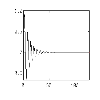
The filter function filters data using a digital filter. The filter is implemented as a direct form II filter which implements the poles first and then the zeros. The difference equation for such a filter is described by the following:
![]()
with a rational system function of

The filter function is called with three or four vectors. The x vector is the data to be filtered and the a and b vectors are the zeroes and poles, respectively. An optional fourth vector, zi, is the initial conditions for the filter state. The filter state is set to zero if zi is not specified.
The output from the filter function is one of two vectors. The first vector, y, is the filtered data. The second vector, zf, is the final state of the filter.
Example:
|
% impulse response b=[0 0.909 0]; a=[1 -0.909 0.818]; x=[1 zeros(1,127)]; y=filter(b,a,x); plot(y); |
|
Related Topics:
Synopsis:
find(expr)
Description:
The find function finds nonzero elements of its argument.
The function returns a column vector with elements which are indices to nonzero elements in its argument.
Remember that in MathViews, matrix indices start at 1 and continue columnwise.
Example:
|
INPUT |
OUTPUT |
| V =
1 2 3 0 4 0 7 |
find(V)
ans = 1 2 3 5 7 |
| A =
1 2 0 0 4 0 6 0 7 |
find(A)
ans = 1 3 4 5 9 |
| A(find(A))
ans = 1 6 2 4 7 |
Related Topics:
Synopsis:
fix(expr)
Description:
The fix function rounds the element(s) of its argument to the nearest integer towards 0.
The argument can be a scalar, a vector, or a matrix.
If the argument has complex element(s), the function operates on both the real and the imaginary parts of the element(s).
Example:
|
INPUT |
OUTPUT |
| A =
-0.3 5.6 4.5 -0.02 5.1 5.6 |
fix(A)
ans = 0 5 4 0 5 5 |
| z = 2.3 + 4.5j |
fix(z)
ans = 2 + 4 j |
Related Topics:
Synopsis:
flip(expr)
Description:
The flip function reverses the order of the rows and columns of its argument.
If the argument is a scalar, the argument is left unchanged.
If the argument is a vector, a column vector of the flipped elements is returned.
If the argument is a matrix, a completely flipped matrix is returned.
Example:
|
INPUT |
OUTPUT |
| A =
1 2 0 0 4 0 6 0 7 9 4 7 |
flip(A)
ans = 7 4 9 7 0 6 0 4 0 0 2 1 |
Related Topics:
Synopsis:
fliplr(expr)
fliplr(expr, ncol)
Description:
The fliplr function reverses the order of the columns of its argument.
If the argument is a scalar, the argument is left unchanged.
If the argument is a vector, a column vector of the flipped elements is returned.
If the argument is a matrix, a complete column flip of the matrix is returned.
If the argument ncol is specified, then only the first ncol columns are used in the flip process.
Example:
|
INPUT |
OUTPUT |
| A =
1 2 0 0 4 0 6 0 7 9 4 7 |
fliplr(A)
ans = 0 2 1 0 4 0 7 0 6 7 4 9 |
| fliplr(A, 2)
ans = 2 1 0 4 0 0 0 6 7 4 9 7 |
Related Topics:
Synopsis:
flipud(expr)
flipud(expr, nrow)
Description:
The flipud function reverses the order of the rows of its argument.
If the argument is a scalar, the argument is left unchanged.
If the argument is a vector, a column vector of the flipped elements is returned.
If the argument is a matrix, a complete row flip of the matrix is returned.
If the argument, nrow, is specified, then only the first nrow rows are used in the flip process.
Example:
|
INPUT |
OUTPUT |
| A =
1 2 0 0 4 0 6 0 7 9 4 7 |
flipud(A)
ans = 9 4 7 6 0 7 0 4 0 1 2 0 |
| flipud(A, -2)
ans = 0 4 0 1 2 0 6 0 7 9 4 7 |
Related Topics:
Synopsis:
floor(expr)
Description:
The floor function rounds the element(s) of its argument to the nearest integer towards .
The argument can be a scalar, a vector, or a matrix.
If the argument has complex element(s), the function operates on both the real and the imaginary parts of the element(s).
Example:
|
INPUT |
OUTPUT |
| A =
-0.3 5.6 4.5 -0.02 5.1 5.6 |
floor(A)
ans = -1 5 4 -1 5 5 |
| z = 2.3 + 4.5j |
floor(z)
ans = 2 + 4 j |
Related Topics:
Synopsis:
format type
Description:
The format function operates on the display format of numbers on the output window. By default, real numbers are displayed in short format. The following table lists the available format types in MathViews.
|
short |
4 digits fixed point |
| long |
15 digits fixed point |
| short e |
4 digits floating point |
| long e |
15 digits floating point |
| hex |
hexadecimal display |
| +, - |
+,- display for values > 0 and < 0 |
| bank |
two digits fixed point |
| compact |
suppresses excess line feeds |
| loose |
airy display |
Example:
|
INPUT |
OUTPUT |
| x = 3.141 |
|
| format short
x |
ans =
3.1410 |
| format long
x |
ans =
3.141000000000000 |
| format short e
x |
ans =
3.1410E+00 |
| format bank
x |
ans =
3.14 |
| A = ones(5,5)
A(2:4, 2:4) = zeros(3,3) A(3,3) = -10 format + A |
A =
+ + + + + + 0 0 0 + + 0 - 0 + + 0 0 0 + + + + + + |
Related Topics:
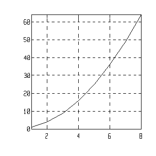
Synopsis:
grid
Description:
Draws grid lines on the currently displayed plot; i.e. the currently active graphics window.
Example:
|
INPUT |
OUTPUT |
| plot(1:8, (1:8).^2)
grid |
|
Related Topics:
plot, hold, title, xlabel, ylabel
Synopsis:
gwclr(win)
Description:
The gwclr function clears a selected graphics window.
If no argument is provided, the command clears the current graphics window.
If an argument is provided, and it is an integer whose value represents the graphics window to be cleared, then the command clears the graphics window indicated by the argument's integer value. The integer value must be less than or equal to the total number of graphics windows selected using gwinit. If an out-of-range window number is referenced, the currently selected graphics window is used for clearing.
Example:
gwclr( 10)
gwclr()
clg
Related Topics:
Synopsis:
gwinit(dimensions, win_titles)
Description:
The gwinit function initializes MathViews accessible windows and their layout on the screen.
The win_titles argument is a array/matrix of N strings, each row represents a title of a MathViews graphics window. The number of rows of win_titles, N, determines the number of preset graphics windows of the current session.
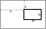
The dimensions argument is an N by 4 matrix, where N is the number of rows in the argument win_titles. Each row of dimensions specifies the location of the graphics window.
The elements of each row must correspond to the following definitions:
The upper left corner of the screen is at location (0,0).
The lower right corner of the screen is at location (1,1)
Each element of a row must be in the range of [0,1] (inclusive).
The elements of each row, [x y wx wy], correspond to the graphical description shown below:
The default allowable number of graphics windows is 8. Range checking is not provided. Also, when resizing graphics windows, be aware that Windows itself puts a constraint on the minimum size of a window.
Example:
A = [ 0.5 0.5 0.2 0.2; .2 .2 .3 .3]
gwinit(A, ['G1'; 'G2'])
Related Topics:
Synopsis:
gwsel(win, dim, title)
Description:
The gwsel function selects a graphics window for graphics display.
The win argument is a real scalar whose value represents the graphics window to be used for displaying a graphic. Win must be less than or equal to the total number of graphics windows selected using gwinit. If an out-of-range window number is referenced, the currently selected graphics window is used.
The dim argument is a 1 by 4 matrix. This argument is used to reassign the location of the selected graphics window. The value of each element in dim follows that described in the gwinit function's dimensions variable. If no reassignment is indicated, an empty matrix must be used in its place.
The title argument retitles the graphics window specified in the argument win.
Example:
gwsel(1, [], 'sin(x)/x)
Related Topics:
Synopsis:
hamming (N)
Description:
This function computes the Hamming windowing function. The argument, N, is the number of samples to be taken.
See the description of the blackman function for additional details on windowing functions.
Example:
|
INPUT |
OUTPUT |
| hamming(5)' |
ans =
0.04 0.52 1 0.52 0.04 |
| plot(hamming(100)) |

|
Related Topics:
hanning, wsina, wmerit, blackman, wbartlet, wrect
Synopsis:
hanning (N)
Description:
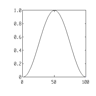
This function computes the Hanning windowing function. The argument, N, is the number of samples to be taken.
See the description of the blackman function for additional details on windowing functions.
Example:
|
INPUT |
OUTPUT |
| hanning(5)' |
ans =
0 0.5 1 0.5 0 |
| plot(hanning(100)) |
|
Related Topics:
hamming, wsina, wmerit, blackman, wbartlet, wrect
Synopsis:
help
help funcname
Description:
The help command displays all the functions currently stored in memory.
If the help command is followed with a funcname, then the funcname is first searched through the directory(ies) in the MathViews path variable for funcname.m. Once found, help will display all the comments following the function keyword up until the first MathViews statement. The M-file must be a function M-file.
If no funcname.m exists then MathViews will search for funcname in the mathview.hlp file. This file must be created using the Cardfile application available in Windows. Be sure to give an index name for each card index. MathViews will use these index names to search for the matching pattern. The user can use this versatile feature to write up his/her own pop-up help files.
Example:
|
INPUT |
OUTPUT |
| help |
MathViews will display a list of built-in
functions. |
Related Topics:
Synopsis:
hilb(norder)
Description:
The hilb function returns an norder by norder Hilbert matrix.
The elements of the Hilbert matrix are defined to be
![]() :
:
Example:
|
INPUT |
OUTPUT |
| hilb(3) |
hilb(3)
ans = 1 0.5 0.333333 0.5 0.333333 0.25 0.333333 0.25 0.2 |
Related Topics:
Synopsis:
hold
hold [on/off]
Description:
The hold function tells MathViews to plot subsequent graphics onto the current graphics window.
Subsequent plots are overlaid onto the plotting area without erasing the current displayed graph. Issuing the command by itself, toggles the current hold mode. The command used with [on/off] explicitly specifies the current hold mode.
MathViews starts with the hold mode off. MathViews will create a new graphics window for each new plot, unless the subplot function or the hold function is used.
When using the hold function, make sure that the domains and ranges of all overlapping plots match. If they do not match, MathViews will create some ambiguous plots.
Example:
|
INPUT |
OUTPUT |
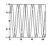
| t = 1:64
plot(t, sin(1.5 * t/pi)) hold on plot(t, cos(1.5 * t/pi)) hold off |
|
Exercise caution when using the hold function. Make sure that all x ranges are the same, otherwise your plot might be ambiguous.
Related Topics:
Synopsis:
home
Description:
The home command clears the current text output functions and puts the cursor at the upper left corner of the window.
Example:
home
Related Topics:
Synopsis:
ifft(expr)
Description:
The ifft function computes the Inverse Fast Fourier Transform (IFFT) of its argument. For additional details, see the discussion on Fourier Transforms in the dft function.
Example:
|
INPUT |
OUTPUT |
| %fft/ifft
subplot(221) x=sinw(16,2)+sinw(16,5)/2 plot(x) y=fft(x) y=abs(fft(x)) plot(y) % should give x y=real(ifft(fft(x))) plot(y) subplot(111) |
|
| y/x |
ans =
16 |
Related Topics:
Synopsis:
imag(expr)
Description:
The imag function extracts the imaginary part of its argument.
If the argument is an array, the function operates on each element of the array. The result is an array with the same dimensions as the argument.
This function is meaningful only for complex arguments. Real arguments are left unchanged.
Example:
|
INPUT |
OUTPUT |
| z = 4 + 5j |
imag(z)
ans = 5 |
| A =
2+4i 10 -3-4i 20 |
imag(A)
ans = 4 0 4 0 |
Related Topics:
Synopsis:
x = input('expr')
Description:
The input function prompts the user for input using the argument as the message prompt.
The function takes scalar and string inputs.
String inputs must begin and end with single quotes. The user input is assigned to x on return.
Example:
x = input('MathViews>')
Related Topics:
Incompatibility with MATLAB:
The form input('expr', 's') is not supported.
Synopsis:
int2str(num)
Description:
The int2str function converts its argument to string format.
Example:
|
INPUT |
OUTPUT |
| x=5;
y=3; ['x+y=' int2str(x+y)] |
['x+y=' int2str(x+y)]
ans = x+y=8 |
Related Topics:
Synopsis:
inv(expr)
Description:
The inv function computes the matrix inverse of its argument.
The argument must be a square and non-singular matrix. A matrix is singular if its determinant is 0. Matrix inversion of complex matrices is also supported.
Example:
|
INPUT |
OUTPUT |
| A =
3 2 2 1 3 4 7 3 2 |
inv(A)
ans = 3 -1 -1 -13 4 5 9 -2.5 -3.5 |
| A * inv(A)
ans = 0 8.88178e-16 0 0 1 0 -3.55271e-15 2.66454e-15 1 |
Notice that this is close to identity. Due to the round-off errors of the computer, 0's can be approximated by very small numbers.
Related Topics:
\ , /
Synopsis:
invhilb(norder)
Description:
The invhilb function computes the inverse of the Hilbert matrix of order norder.
Computing the inverse of a Hilbert matrix is a well-posed problem. As the order increases, the Hilbert matrix becomes more and more ill-conditioned.
Example:
|
INPUT |
OUTPUT |
| hilb(5) |
ans =
1 0.5 0.333333 0.25 0.2 0.5 0.333333 0.25 0.2 0.166667 0.333333 0.25 0.2 0.166667 0.142857 0.25 0.2 0.166667 0.142857 0.125 0.2 0.166667 0.142857 0.125 0.111111 |
| cond(hilb(5)) |
cond(hilb(5))
ans = 476607 |
Related Topics:
Synopsis:
iscmplx(expr)
Description:
The iscmplx function tests whether the contents of its argument is(are) complex numbers.
If any of the elements of the argument is(are) complex, the function returns a 1. If none of the elements of the argument is(are) complex, then the function returns a 0.
Example:
|
INPUT |
OUTPUT |
| z = 2+3i
A = [ 2 i; 0 3] |
iscmplx(z)
ans = 1 |
| iscmplx(A)
ans = 1 |
Related Topics:
Synopsis:
iscol(expr)
Description:
The iscol function returns a logical value based on the type of it argument.
If the argument is a column vector, a 1 is returned; otherwise a 0 is returned.
Example:
|
INPUT |
OUTPUT |
| A =
2 3 4 |
|
| if iscol(A)
disp('A is a column vector') end |
A is a column vector |
Related Topics:
isreal, isvector, iscmplx, isrow
Synopsis:
isempty(expr)
Description:
The isempty function tests its argument for an empty value.
The function returns 1 if its argument is an empty argument; otherwise a 0 is returned.
An empty matrix is of the form A = [].
Example:
|
INPUT |
OUTPUT |
| A = [] |
isempty(A)
ans = 1 |
| B =
3 4 4 5 |
isempty(B)
ans = 0 |
Related Topics:
isreal, isvector, isrow, iscol
Synopsis:
isreal(expr)
Description:
The isreal function returns a logical value based on the type of its argument.
If the argument is a scalar value, a 1 is returned; otherwise a 0 is returned.
Example:
|
INPUT |
OUTPUT |
| A = 2 |
|
| if isreal(A)
disp('A is a scalar') end |
A is a scalar |
Related Topics:
iscol, isvector, iscmplx, isrow
Synopsis:
isrow(expr)
Description:
The isrow function returns a logical value based on the type of its argument.
If the argument is a row vector, a 1 is returned; otherwise a 0 is returned.
Example:
|
INPUT |
OUTPUT |
| A =
2 3 4 |
|
| if isrow(A)
disp('A is a row vector') end |
A is a row vector |
Related Topics:
iscol, isvector, iscmplx, isreal
Synopsis:
isscalar(expr)
Description:
The isscalar function returns a logical value based on the type of its argument.
If the argument is a scalar, a 1 is returned; otherwise a 0 is returned.
Example:
|
INPUT |
OUTPUT |
| A =
2 3 4 |
|
| if isscalar(A)
disp('A is a scalar') end |
(returns nothing; A is not a scalar) |
Related Topics:
Synopsis:
isstr(expr)
Description:
The isstr function returns a 1 if its argument is a string; otherwise a 0 is returned.
Example:
|
INPUT |
OUTPUT |
| str = 'MathViews' |
isstr(str)
ans = 1 |
| num = 4 |
isstr(num)
ans = 0 |
|
isstr(abs(str)) ans = 0 |
The test is 0 because abs(str) converts str into the integer equivalent of the ASCII string. Thus str is no longer an ASCII string.
Related Topics:
Synopsis:
isvector(expr)
Description:
The isvector function returns a logical value based on the type of its argument.
If the argument is a vector, a 1 is returned; otherwise a 0 is returned.
Example:
|
INPUT |
OUTPUT |
| A =
2 3 4 |
|
| if isvector(A)
disp('A is a vector') end |
A is a vector |
Related Topics:
Synopsis:
keyboard
Description:
The keyboard command relinquishes control, during the execution of an M-file, to the interactive window for input.
After issuing the command, all other MathViews commands are valid. To exit this interactive command mode and return to the M-file for subsequent processing, type ctrl-z in the interactive window.
Example:
keyboard
Related Topics:
Synopsis:
length(expr)
Description:
The length function returns the length of it argument, i.e. max( size(expr)).
Example:
|
INPUT |
OUTPUT |
| str = 'MathViews' |
length(str)
ans = 9 |
| num = 4 |
length(num)
ans = 1 |
| A =
1 2 3 4 3 2 |
length(A)
ans = 3 |
Related Topics:
Synopsis:
load filename
Description:
The load command loads an MAT-file into MathViews' memory.
If no filename is given, then the default mathviews.mat is loaded into memory, provided mathview.mat exists; otherwise, nothing is done.
MAT-files can only be generated using the save command.
Complete DOS pathnames can be used to access '.mat' files. Long file names (LFN) are supported. If the LFN contains
Example:
save test
clear
load test
Saves the current contents in memory on disk file 'test.mat' (MathViews inserts the extension '.mat' if one is not provided); clears the contents of memory; loads into memory the variables stored in diskfile 'test.mat'.
Related Topics:
Synopsis:
log(expr)
Description:
The log function computes the natural log of its argument.
If the argument is an array, the function operates on each element of the array. The result is an array with the same dimensions as the argument.
If the argument has complex element(s), the complex logarithm:
![]()
is used to compute the result.
Example:
|
INPUT |
OUTPUT |
| z = 3 + 2i
log(z) |
ans =
1.28247 + 0.588003 j |
| log(abs(z)) + i *atan2(imag(z),real(z))
|
ans = 1.28247 + 0.588003 j |
Related Topics:
atan2, atan, sin, cos, real, imag, abs, exp, log
Synopsis:
log2(expr)
Description:
The log2 function computes the base 2 log of its argument.
If the argument is an array, the function operates on each element of the array. The result is an array with the same dimensions as the argument.
This function also supports complex arguments in general, and negative numbers in particular.
The function is not defined for 0 values.
Example:
|
INPUT |
OUTPUT |
| log2([64 512 1024]) |
ans =
6 9 10 |
Related Topics:
Synopsis:
log10(expr)
Description:
The log10 function computes the base 10 log of its argument.
If the argument is an array, the function operates on each element of the array. The result is an array with the same dimensions as the argument.
This function also supports complex arguments in general, and negative numbers in particular.
The function is not defined for 0 values.
Example:
|
INPUT |
OUTPUT |
| log10(100) |
ans =
2 |
Related Topics:
Synopsis:
loglog(data)
loglog(data1, data2)
Description:
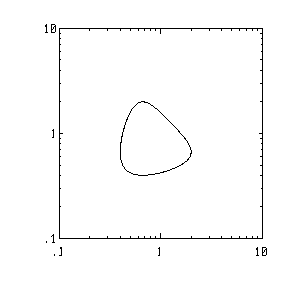
The loglog function generates log-log line plots.
If one argument is provided and is a vector, then each element is plotted vs. its relative index in the vector. However, if the argument is a matrix, each column is used to generated multiple plots using the scheme described for vectors.
If a second argument is provided, the dimensions of both arguments must be equal. In this case, each element of each column in the first argument is plotted vs. each element of each column in the second argument.
Example:
|
INPUT |
OUTPUT |
| x = 0:.1:8*pi
loglog(1/(x->sin+1.5),1/(x->cos+1.5)) |
|
Related Topics:
Synopsis:
ltifr(a,b,s)
Description:
The ltifr function is used to generate a kernel for propataging the frequency response of linear time-invariant systems. The frequency response is computed as:
![]()
where s represents the complex frequencies at which to compute the frequency response. The inputs a and b are the state-space representation of the linear time-invariant system.
Example:
|
G = ltifr(a,b,s) Return the frequency response in G for the system represented by a
and b. |
Related Topics:
Synopsis:
ltitr(a,b,u)
ltitr(a,b,u,x0)
Description:
The ltitr function is used to generate a kernel for propataging the time response of linear time-invariant systems. The input parameters a and b are the state-space representation of the system. U is the points in time at which to compute the response. X0 can be used to set the initial conditions of the states.
Example:
|
y = ltitr(a,b,u) Return the kernel for the system reperesented by a and b in y. |
Related Topics:
Synopsis:
max(expr)
max(expr1,expr2)
[maxV, maxI] = max(expr)
Description:
The max function finds the maximum value of the argument.
If the argument is a vector, the largest element of the vector is returned.
If the argument is a matrix, then the function operates on each column, returning a row vector with elements pertaining to the max of each column.
If the max function is called with two arguments, the dimensions of the
two arguments must be equal, and the dimensions of the return value are
equal to those of the arguments. With two arguments, the function operates
on elements of the arguments. For example: C = max(A,B), then
![]() .
.
In addition, for single argument invocations, an index vector can be obtain, which indicates the index of the maximum element within the original matrix.
Example:
|
INPUT |
OUTPUT |
| A =
1 10 1 10 1 10 max(A,B) |
ans =
10 10 10 10 10 10 |
| B =
10 1 10 1 10 1 max(A) |
ans =
10 10 10 |
| [V,I] = max(A) |
V = 10 10 10 I = 2 1 2 |
Related Topics:
Synopsis:
mean(expr)
Description:
The mean function calculates the average of its argument.
If the argument is a vector, the mean is the average of the argument's elements.
If the argument is a matrix, the mean is computed columnwise, returning a row vector with elements being the mean of each corresponding column of the argument.
The mean of complex vectors is not supported.
Example:
|
INPUT |
OUTPUT |
| A =
1 10 1 10 1 10 mean(A) |
ans =
5.5 5.5 5.5 |
Related Topics:
Synopsis:
median(expr)
[A, I] = median(expr)
Description:
The function median returns the median of the contents of its argument.
If the argument is a vector, the function calculates the median of the vector's elements.
If the argument is a matrix, the median is computed columnwise, returning a row vector whose elements are the median of each column.
If the I parameter is given, the index of the median in the original array is also returned.
If the input argument is a matrix, then I is a row vector with elements being the index of the median in each column of the original matrix.
The median function uses the (n/2 + 1)th element when n is even.
Example:
|
INPUT |
OUTPUT |
| v =
6 4 10 34 67 3 15 median(v) |
ans =
10 |
| M =
1 2 3 4 8 3 4 3 10 23 4 1 [V, IND] = median(M) |
V =
8 3 4 3 IND = 2 2 3 2 |
Related Topics:
Synopsis:
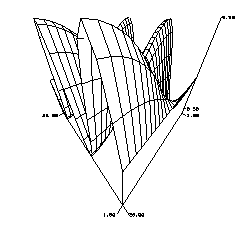
mesh(data)
mesh(data, [z theta phi], [xs ys zs], [xrange], [yrange])
Description:
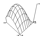
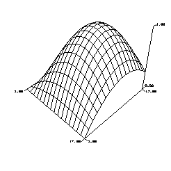
The mesh function generates a hidden-lines plot.
The argument must be a 2-dimensional array, i.e. a matrix. The data values in the argument indicate the heights above the X-Y plane.
The function can also be used to change the viewing orientation of the plot.
The extra parameters have the following meanings:
|
z |
viewing distance from the object. |
| theta |
angle of rotation relative to the XY plane in degrees
|
| phi |
angle of rotation relative to the Z axis |
| xs, ys, zs |
XYZ axis scale parameters in integers |
| xrange, yrange |
the number of points in the X, Y range. (Note: this
set of numbers can't exceed the number of columns of data.)
|
(next page)
Example:
|
INPUT |
OUTPUT |
| n=8;
x=(0:n)/n; y=x.*(1.2-x); y /= max(y); z=y'*y; mesh(z) |
|
| mesh(z, [4 135 135],[1 1 1],[1:17],[1:17])
|
|
Related Topics:
Synopsis:
[X,Y] = meshdom(expr1, expr2)
Description:
The meshdom function generates 2D arrays, X and Y to be used to generate data for the mesh function.
The two input arguments must be vectors of equal dimensions.
Example:
|
INPUT |
OUTPUT |
| x = 0:.5:4*pi;
y = 0:.5:4*pi; [XX,YY]=meshdom(x,y); ZZ = 0.5*sin(XX).*cos(YY./4); mesh(ZZ) |
|
Related Topics:
Synopsis:
meta
meta filename
Description:
The meta function creates a Windows metafile(wmf) for storing the graphics output in the currently active graphics window.
If the command is used alone, the default metafile is 'mvmeta.wmf'; otherwise, the specified filename is used. MathViews will insert the '.wmf' extension if it is not explicitly given. The files saved will be placed in MathViews startup directory, unless a full pathname is given.
The startup directory is specified through the properties option under Windows.
Example:
meta
meta mygraphs
Related Topics:
Synopsis:
min(expr)
min(expr1,expr2)
[minV, minI] = min(expr)
Description:
The min function finds the minimum value of the argument.
If the argument is a vector, the smallest element is returned.
If the argument is a matrix, then the function operates on each column, returning a row vector with elements pertaining to the minimum element of each column.
If the min function is called with two arguments, then the
dimensions of the two arguments must be equal, and the dimensions of the
return value are equal to those of the arguments. With two arguments, the
function operates on elements of the arguments. For example: C =
min(A,B), then ![]() .
.
In addition, for single-argument invocations, an index vector can be obtained, which indicates the index of the minimum element within the original matrix.
Example:
|
INPUT |
OUTPUT |
| A =
1 10 1 10 1 10 min(A,B) |
ans =
1 1 1 1 1 1 |
| B =
10 1 10 1 10 1 min(A) |
ans =
1 1 1 |
| [V,I] = max(A) |
V =
1 1 1 I = 1 2 1 |
Related Topics:
Synopsis:
norm(expr)
norm(expr, p)
Description:
The norm function computes the vector or matrix norm of its argument.
If the argument is a vector, the following equation is used to compute the vector norm:
sum(abs(expr).^)^(1/p)
If the argument is a matrix, the following equation is used to compute the matrix norm when p == 1:
max(sum(abs(real(expr))+abs(imag(expr))).
When p == 2, then the norm of the matrix is the largest singular value of the argument.
If p is not specified, p is assumed to be 2.
Example:
|
INPUT |
OUTPUT |
| x = 1:10
A =[ 1 1 2; 2 4 -3; 3 6 -5] norm(x) |
ans =
19.62 |
| norm(A) |
ans = 9.948 |
|
norm(A,1) |
ans = 11 |
Related Topics:
Synopsis:
str = num2str(num)
Description:
The num2str function converts a number into a string array.
Example:
|
INPUT |
OUTPUT |
| x=5.551;
y=3.63; ['x+y=' num2str(x+y)] |
ans =
x+y=9.181 |
Related Topics:
Synopsis:
ones(expr)
ones(expr1, expr2)
Description:
The ones function returns an array with all 1's as its elements.
If the argument(s) is(are) integers, the function returns an expr by expr matrix(expr1 by expr2 matrix).
If the argument is an array, then the result is an array with the same dimensions as the argument. The function returns a matrix with 1's for its elements.
Example:
|
INPUT |
OUTPUT |
| A =
1 10 1 10 1 10 ones(A) |
ans =
1 1 1 1 1 1 |
| ones(3) |
ans =
1 1 1 1 1 1 1 1 1 |
| ones(4,5) |
ans = 1 1 1 1 1 1 1 1 1 1 1 1 1 1 1 1 1 1 1 1 |
Related Topics:
Synopsis:
pack
Description:
This function is provided to for compatiblity with MATLAB. It does nothing. MathViews uses the excellent Windows memory management system. MathViews handles the details of memory management and you should not have to worry about using pack to handle compaction of memory.
Example:
pack
Related Topics:
Synopsis:
pause
pause(expr)
Description:
The pause function causes an M-file to pause for a moment.
If the command is used without an argument, a 1-second pause is initiated.
If an argument is specified, the argument must be an integer representing the length of the pause in seconds. The function waits for argument-value of seconds before continuing. In MathViews, pause is discontinued by clicking on the OK button.
Example:
sec = 5
pause (sec)
Related Topics:
Synopsis:
pi
Description:
The pi function returns as a function rather than a constant. By using the function, the value cannot be cleared, whereas if it were declared as a constant it could be cleared.
Example:
not applicable
Related Topics:
not applicable
Synopsis:
pinv(expr)
Description:
The pinv function computes the Moore-Penrose pseudo-inverse of a nonsquare matrix.
Example:
|
INPUT |
OUTPUT |
| a=[1 2 3; 4 3 2];
pinv(a) |
ans =
-0.2333 0.2667 0.06667 0.06667 0.3667 -0.1333 |
| a*pinv(a) |
ans =
1 0 0 1 |
Related Topics:
Synopsis:
play( filename)
Description:
The play function displays a Windows metafile onto a new MathViews graphics window.
The argument filename must be contained in single quotes. MathViews will only search for the file in the startup directory unless a full path is given in the filename argument.
Example:
play('mvmeta.wmf')
play('C:\EXAMPLE\pic.wmf')
Related Topics:
Synopsis:
plot (expr)
plot( [expr1, expr2, 'format',] ...)
Description:
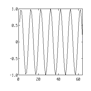
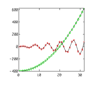
The plot function generates 2-dimensional line plots.
If the argument is a vector, each element of the vector is plotted vs. its index. If two arguments are provided, they must have the same dimensions. Then argument 1 is the domain and argument 2 is the range.
If both arguments are 2-dimensional arrays, they must have the same dimensions. Then each column of the first argument is plotted vs. the corresponding column in the second argument.
The user can also specify the line type or symbol type and color of the line plot. The format is specified in between single quotes. For example, '+r' means use the plus(+) as symbol and use the color red for the symbol.
|
Symbol Types |
Line Types |
Color |
| point(.) |
solid(-) |
red |
| plus(+) |
dashed(- -) |
green |
| star(*) |
dotted(. .) |
blue |
| circle(o) |
dash-dot(-.) |
|
| x-mark(x) |
Example:
|
INPUT |
OUTPUT |
| t = 1:64
plot(t, sin(2*t/pi)) |
|
| t = 0:32
t2 =-400 + t^2; t4 = 4*t.*sin(t); plot(t,t2,'+g',t,t4,'*r') hold on plot(t,t2,t,t4) hold off |
|
Related Topics:
Description:
polar(angle, radius)
Description:
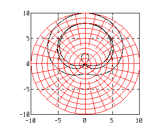
The polar function generates a polar plot of its arguments.
The polar function takes two arguments; the first argument specifies the angle and the second argument specifies the length of the vector at that angle.
If the two arguments are vectors, the number of elements of each argument must be the same.
If the two arguments are matrices, then the dimensions of the two arguments must be the same. In addition, the polar plots generated are computed columnwise.
The grid function on a polar plot will generate a polar grid.
Example:
|
INPUT |
OUTPUT |
| pi = acos(-1);
theta=0:.1:4*pi; r=4+4*sin(theta); r1=3+5*sin(theta); r2 = 6+4*sin(theta); polar(theta,r2); hold on polar(theta,r1); polar(theta,r); grid |
|
Related Topics:
Synopsis:
poly(expr)
Description:
The poly function computes the characteristic polynomial of a square matrix or the polynomial coefficients of a roots vector.
Example:
|
INPUT |
OUTPUT |
| r = [3 2 -1 -1]
poly(r) |
ans = 1 -3 -3 7 6 |
Related Topics:
Synopsis:
p = polyfit(v1, v2, np)
Description:
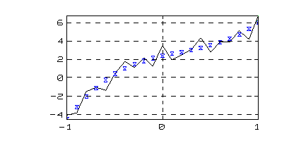
The polyfit function computes a polynomial fit in the least squares sense of its arguments. Given vector v1, polynomial np(x) fits vector v2.
Example:
|
INPUT |
OUTPUT |
| p=[1 3 -3 2 1]
x=-1:0.1:1; y=polyval(p,x)+3*rand(x); % 3-order polynomial pe=polyfit(x,y,3) ye=polyval(pe,x); |
p =
1 3 -3 2 1 pe = 2.879 -1.622 2.376 2.376 |
| plot(x,y,x,ye,'x'),grid |
|
Related Topics:
Synopsis:
polyval(p, x)
Description:
The polyval function evaluates the polynomial, p, at the specific values of x.
Example:
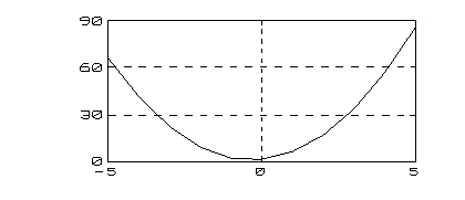
The polynomial p(s) = 3s2+ 2s+1 is evaluated at s = 5 as follows
|
INPUT |
OUTPUT |
| p = [3 2 1];
polyval(p,5) |
ans =
86 |
| x=-5:5;
plot(x,polyval(p,x))grid |
|
Related Topics:
Synopsis:
prtsc
Description:
The print/prtsc functions print the image on the current MathViews graphics window.
Printing the image in a MathViews graphics window can also be done using the print option in the graphics window's control menu.
The printer setup is done through Window Control Panel.
Example:
prtsc
Related Topics:
Synopsis:
prod(expr)
Description:
The prod function computes the product of its argument's elements.
If the argument is a vector, the function computes the product of the argument's elements.
If the argument is a matrix, the function computes the product of each column of the argument. It returns a row vector who's elements are the products of each corresponding column of the argument.
Example:
|
INPUT |
OUTPUT |
| A =
1 2 3 4 5 prod(A) |
ans = 120 |
| B =
2 3 4 4 5 6 5 6 7 prod(B) |
ans =
40 90 168 |
Related Topics:
Synopsis:
[Q,R]=qr(A)
Description:
The qr function computes the QR factorization of a nonsquare matrix.
The argument, A, is an (m,n) matrix. Q is a unitary (m,m) matrix, i.e. QTQ=I, and R is an upper triangular (m,n) matrix such that A=Q*R;
Example:
|
INPUT |
OUTPUT |
| a=[1 2 3; 4 3 2];
QR=qr(a) |
Q =
-0.2425 -0.9701 -0.9701 0.2425 R = -4.1231 -3.3955 -2.6679 0.0000 -1.2127 -2.4254 |
| Q*Q |
ans =
1 0 0 1 |
Related Topics:
Synopsis:
rand(expr)
rand(expr1, expr2)
seed = rand('seed')
rand('seed', newseed)
Description:
The rand function generates random numbers.
If the argument is an integer, an expr by expr matrix is generated, with elements being random numbers in the range of (0,1).
If the argument is a matrix, the function will generate a matrix with dimensions equal to that of the argument; the resulting matrix contains randomly generated elements.
If two arguments are used to invoke the function, both arguments must be integers. The function will generate an expr1 by expr2 random elements matrix.
rand('seed') returns the current seed. rand('seed', 0) reset the seed to zero
Example:
|
INPUT |
OUTPUT |
| rand(3) |
ans =
0.209985 0.194112 0.306115 0.266308 0.697822 0.418132 0.37338 0.0412352 0.537115 |
| rand(3,2) |
ans =
0.11756 0.107433 0.2034 0.678925 0.562707 0.0745257 |
| B =
2 3 4 4 5 6 |
rand(B)
ans = 0.300326 0.819378 0.976426 0.242718 0.585383 0.405369 |
Related Topics:
Incompatibilities with MATLAB:
rand('dist') and rand('normal') are supported in MathViews.
Synopsis:
randn(expr)
randn(expr1, expr2)
seed = randn('seed')
randn('seed', newseed)
Description:
The randn function generates random numbers.
If the argument is an integer, an expr by expr matrix is generated, with elements being random numbers with normal distribution.
If the argument is a matrix, the function will generate a matrix with dimensions equal to that of the argument; the resulting matrix contains randomly generated elements.
If two arguments are used to invoke the function, both arguments must be integers. The function will generate an expr1 by expr2 random elements matrix.
randn('seed') returns the current seed. randn('seed', 0) reset the seed to zero
Example:
|
INPUT |
OUTPUT |
| randn(3) |
ans =
0.6391 -0.1097 2.0099 1.1099 -1.2400 -1.2951 0.7092 0.7046 0.2839 |
| randn(2,3) |
ans =
-1.4185 1.1077 -2.4968 -0.1838 0.4996 -0.8039 |
Related Topics:
Synopsis:
rank(expr)
rank(expr, tol)
Description:
The rank function computes the rank of a matrix.
The rank of a matrix is the number of linearly independent columns of the matrix. For example, if a matrix A(mxn) has full rank, then the only vector X(nx1) that will satisfy AX = 0 is the vector X = 0.
Example:
|
INPUT |
OUTPUT |
| A =
1 1 2 2 4 -3 3 6 -5 rank(A) |
ans = 3 |
|
rank(A') |
ans =
3 |
Related Topics:
Synopsis:
rcond(expr)
Description:
The rcond function computes the reciprocal of the condition number of its argument in 1-norm.
If the argument is a matrix, the argument must be a square matrix. The function computes the reciprocal of the condition number of the argument. The condition number is the sensitivity of the solution of a system of linear equations to errors in data.
When this number is near 1, the matrix is said to well conditioned. If this number is close to 0, the matrix is said to be ill conditioned.
Example:
|
INPUT |
OUTPUT |
| A =
1 0.99 0.99 0.98 rcond(A) |
ans = 2.538e-05 |
| cond(A) |
ans = 3.921e+04 |
Obviously, matrix A is ill conditioned.
Related Topics:
Synopsis:
real(expr)
Description:
The real function extracts the real part of its argument.
If the argument is an array, the function operates on each element of the array. The result is an array with the same dimensions as the argument.
This function is meaningful only for complex arguments, real arguments are left unchanged.
Example:
|
INPUT |
OUTPUT |
| z = 4 + 5j
real(z) |
ans = 4 |
| A =
2+4i 10 -3-4i 20 real(A) |
ans =
2 10 -3 20 |
Related Topics:
Synopsis:
rem(expr1, expr2)
Description:
The rem function computes the remainder of the two arguments.
The function returns the remainder of expr1./expr2, i.e.
expr1 - expr2 * fix(expr1./expr2).
If complex arguments are used, the complex parts are ignored.
If the arguments are matrices, the arguments must have the same dimensions. The function operates on individual elements.
Example:
|
INPUT |
OUTPUT |
| z1 = 7 + 4j
z2 = 5 + 3j rem(z1, z2) |
ans =
2 |
Notice that only the real part is used in the computation.
Related Topics:
/, \
Synopsis:
bVec=remez(nCoeff, vFreq, vDesiredResponse, vWeight, 'fType')
bVec=remez(nCoeff, vFreq, vDesiredResponse)
Description:
The remez computes the nCoeff+1 coefficients of a digital finite-impulse response (FIR) filter using the Parks-McClellan algorithm. Such digital FIR filters are referred to as equi-ripple digital filters.
Example:
|
INPUT |
OUTPUT |
| nCoeff = 59;
vFreq = [0 0.16 0.199 0.201 0.24 0.5]; vDesiredResponse = [0 0 1 1 0 0]; vWeight = [1 1 1]; bVec = remez(nCoeff, vFreq,vDesiredResponse, vWeight) n = 512 ; [yf, xf]= freqz(bVec, 1, n); plot(vFreq,vDesiredResponse,xf/pi,yf) |
Related Topics:
Synopsis:
reshape(expr1,rows, cols)
Description:
The reshape function is used to reshape an array.
The resulting array must have the same number of elements as the original array, i.e. expr1. Thus, the prod( [ rows cols]) must equal that of prod( size(expr1)). The reshaping process operates columnwise.
Example:
|
INPUT |
OUTPUT |
| A =
1 2 3 4 3 4 5 6 7 6 5 4 A = reshape(A, 2, 6) |
A = 1 7 4 3 5 6 3 2 6 5 4 4 |
Related Topics:
Synopsis:
roots(p)
Description:
The roots function computes the roots of a polynomial. The vector p represents the coefficients of the polynomial as follows:
![]()
Example:
Consider solving the roots for equation: ![]()
|
INPUT |
OUTPUT |
| p := [1 -3 -3 7 6] |
r = roots(p)
r = 3 2 -1 + 6.294e-09 j -1 - 6.294e-09 j |
Related Topics:
Synopsis:
round(expr)
Description:
The round function rounds element(s) of its argument to the nearest integer.
The argument can be a scalar or an array.
If the argument has complex element(s), the function operates on both the real and the imaginary parts of the element(s).
Example:
|
INPUT |
OUTPUT |
| A =
-0.3 5.6 4.5 -0.02 5.1 5.6 round(A) |
ans = 0 6 5 0 5 6 |
| z = 2.3 + 4.5j
round(z) |
ans =
2 + 5j |
Related Topics:
Synopsis:
save filename
save filename var1 var2 ... /ascii/double
Description:
The save command saves the current memory items into a .MAT file. The optional parameters, /ascii and /double, can be used to modify how data is stored. The /ascii parameter tells MathViews to store the data as ASCII values, rather than as binary data. The /double command specifies that numbers are formatted using 16 character digits rather than the default 8 character digits.
The save command is a MathViews command that saves MathViews variables onto disk for storage and retrieval.
If save is used without the filename argument, then MathViews saves the variables to a default file named 'mathvus.mat'.
Example:
save test
clear
load test
Saves the current contents in memory on disk file 'test.mat' (MathViews inserts the extension '.mat' if one is not provided); clears the contents of memory; loads into memory the variables stored in diskfile 'test.mat'.
Related Topics:
Synopsis:
semilogx(data)
semilogx(data, expr2)
Description:
The semilogx and semilogy functions generate semilog line plots.
If the argument is a vector, then each element is plotted vs. its relative index in the vector.
If the argument is a matrix, each column is used to generated multiple plots using the scheme described for vectors.
If the second argument is provided, the dimension of the first and the second arguments must be the same. In this case, each element of each column in the first argument is plotted vs. each element of each column in the second argument.
Semilogy is used similarly, except that the log is on the y axis.
Example:
|
INPUT |
OUTPUT |
| x=0:.1:4*pi;
x = [ x' x']; semilogx(x) grid xlabel('log in X-axis') |

|
Related Topics:
Synopsis:
setstr(expr)
Description:
The setstr function sets the content(s) of its argument to ASCII characters.
Example:
|
INPUT |
OUTPUT |
| t = 'MathViews'
setstr(abs(t)) |
ans =
MathViews |
Related Topics:
Synopsis:
sign(expr)
Description:
The sign function computes the sign of its argument.
The function returns 1 for positive arguments, -1 for negative arguments, and 0 for arguments of 0 value.
If the argument is an array, the function operates on each element of the array, and the result is an array of the same dimensions as the argument.
If the argument has complex elements, then sign returns expr./ abs(expr)
Example:
|
INPUT |
OUTPUT |
| A =
2 -1 -3 0 0 3 sign(A) |
ans =
1 -1 -1 0 0 1 |
| z = 4 + 5j
sign(z) |
ans =
0.624695 + 0.780869 j |
Note that this answer is exactly z./abs(z).
Related Topics:
Synopsis:
sin(expr)
Description:
The sin function computes the sine of its argument, returning a value in radians.
If the argument is an array, the function operates on each element of the array. The result is an array with the same dimensions as the argument.
If the argument has complex elements, then the complex cosine function:
![]()
is used to compute the result.
Example:
|
INPUT |
OUTPUT |
| z = 3 + 4j |
sin(z)
ans = 3.85374 + 27.0168j |
Related Topics:
Synopsis:
sinh(expr)
Description:
The sinh function computes the hyperbolic sine of its argument.
If the argument is a array, the function operates on each element of the array. The result is an array with the same dimensions as the argument.
Example:
|
INPUT |
OUTPUT |
| z = 3 + 4j |
sinh(z)
ans = -6.54812 - 7.61923 j |
Related Topics:
Synopsis:
sinw(points, cycles, freq, phase)
Description:
The sinw function is used to create sinusoidal waveforms.
The arguments are:
|
points |
number of elements of the waveform sequence |
| cycles |
the number of cycles of the waveform |
| freq |
the frequency deviation of the waveform |
| phase |
the initial phase of the waveform |
The sinw function is identical to the cosw function except that the default value of the initial phase is ninety degrees rather than 0.
Example:
See the cosw example.
Related Topics:
Synopsis:
[m,n] = size(expr)
m = size(expr, 1)
n = size(expr, 2)
Description:
The size function returns the size of its argument.
If the argument is a scalar, the function returns the value unity.
If the argument is an array, the function returns the number of rows and the number of columns as: a row vector of two elements.
The function size(A,1) returns the number of rows of A.
The function size(A,2) returns the number of columns of A.
Example:
|
INPUT |
OUTPUT |
| [m,n] = size(3) |
m = 1 n = 1 |
| A =
2 -1 -3 0 0 3 size(A) |
ans =
2 3 |
Related Topics:
Synopsis:
sort(expr)
[X,I] = sort(expr)
Description:
The sort function sorts the contents of its argument.
If the argument is a vector, the function sorts the vector in ascending order.
If the argument is a matrix, the function sorts the argument columnwise in ascending order.
The function also returns a matrix of indices of the original order of the argument.
If the argument has complex elements, the function operates on the absolute value of the elements.
Example:
|
INPUT |
OUTPUT |
| A =
5 32 3 1 2 8 37 1 4 3 [X,I]=sort(A) |
X = 5 32 1 1 2 8 37 3 4 3 I = 1 1 2 1 1 2 2 1 2 2 |
| Z =
3 + 8 j 3 + 7 j 3 + 8 j 2 + 8 j sort(Z) |
ans =
3 + 8 j 3 + 7 j 3 + 8 j 2 + 8 j |
Related Topics:
Synopsis:
sqrt(expr)
Description:
The sqrt function computes the square root of its argument.
If the argument is an array, the function operates on each element of the array. The result is an array with the same dimensions as the argument.
This function also supports complex arguments in general, and it supports negative numbers in particular.
Example:
|
INPUT |
OUTPUT |
| z = -1 |
sqrt(x)
ans = i |
| x =
3 4 |
sqrt(x)
ans = 1.73205 2 |
Related Topics:
Synopsis:
startup
Description:
The startup.m file is invoked every time MathViews starts up. The user can put all his most commonly used constants assignments in the startup.m files.
The _MVPATH variable can also be initialize in the startup.m file.
Example:
startup
Related Topics:
Synopsis:
strcmp(s,t)
Description:
The strcmp function compares its two arguments, s and t, and returns 1 if they are equal, 0 otherwise.
Example:
|
INPUT |
OUTPUT |
| s='Math';
strcmp(s,'math') |
ans =
0 |
| strcmp(s,'Math') |
ans =
1 |
| strcmp(s,'MathViews') |
ans =
0 |
| strcmp(s,6) |
ans =
0 |
Related Topics:
Synopsis:
subplot
subplot(mnq)
Description:
The function subplot creates smaller subplot windows on the current graphics window. The 'mnq' parameters specify the number and positions of the smaller subplot windows within the graphics window, and also specify the current subplot window. The m parameter stands for the number of subplots vertically, and the n for number of subplots horizontally within the major window.
In the Direct Address Mode, the q parameter indicates the current subplot window for the plot. In the Auto Increment Mode, the q parameter indicates the starting subplot window for the plots.
The parameters mnq must be concatenated forming an integer. The limits are 0 m, n 9 and q m n.
To disable the subplot function, use 111 as the input argument (indicating one window vertically, one window horizontally, and plot in window 1).
Example:
|
INPUT |
OUTPUT |
| t = 1:8
subplot(221) plot(t, t.^2) plot(t, t.^0.5) plot(t, t.^3/2) plot(t, t.^6) |
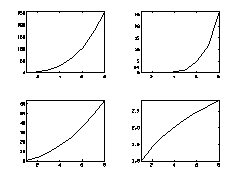
|
Related Topics:
plot, semilogx, semilogy, mesh, contour
Synopsis:
sum(expr)
Description:
The sum function computes the sum of all the elements of its argument.
If the argument is a vector, the function computes the total sum of the vector.
If the argument is a matrix, the function computes the sum of each column of the argument, returning a row vector with elements that are the sums of each column of the argument.
Example:
|
INPUT |
OUTPUT |
| A =
5 32 3 1 2 8 37 1 4 3 sum(A) |
ans =
13 69 4 5 5 |
| Z =
3 + 8 j 3 + 7 j 3 + 8 j 2 + 8 j sum(Z) |
ans =
6 + 16 j 5 + 15 j |
Related Topics:
Synopsis:
svd(expr)
[U,D,V] = svd(expr)
[U,D,V] = svd(expr, 0)
Description:
The svd function computes the singular values of a matrix.
If a return variable is not given, then only a vector of the singular values of expr is returned if the solutions converge. If the U, D, V return variables are given, then both U and V are unitary matrices and D is the diagonal matrix of the singular values of expr. The singular values in D are arranged in decreasing order, D(1,1) being the largest.
If the second argument of the svd function is given ( it must be a 0), then the columns of U = min(size(D)).
(next page)
Example:
|
INPUT |
OUTPUT |
| A =
1 -1 -2 1 0 2.44949 1 1 svd(A) |
ans =
3.16228 2.23607 |
| [U,S,V]=svd(A) |
U = 0.424264 -0.2 0.872697 0.135644 -0.565685 0.6 0.342542 0.450183 -0.69282 -0.489898 0.293028 -0.440607 -0.141421 -0.6 -0.187614 0.764723 S = 3.16228 0 0 2.23607 0 0 0 0 V = 0.447214 -0.894427 -0.894427 -0.447214 |
Related Topics:
Synopsis:
tan(expr)
Description:
The tan function computes the tangent of its argument, returning a value in radians.
If the argument is an array, the function operates on each element of the array. The result is an array with the same dimensions as the argument.
Tangents of complex numbers and arrays are also supported.
The value of tan(x) at its "singular points" is undefined.
Example:
|
INPUT |
OUTPUT |
| z = 4 + 5i
tan(z) |
ans =
8.98348e-05 + 1.00001 |
| sin(z)/cos(z) |
ans = 8.98348e-05 + 1.00001 j |
Related Topics:
Synopsis:
tanh(expr)
Description:
The tanh function computes the hyperbolic tangent of its argument.
If the argument is an array, the function operates on each element of the array. The result is an array with the same dimensions as the argument
The hyperbolic tangent function supports complex arguments.
Example:
|
INPUT |
OUTPUT |
| z = 4 + 5i
tanh(z) |
ans = 1.00056 - 0.000365203 j |
| sinh(z)/cosh(z) |
ans = 1.00056 - 0.000365203 j |
Related Topics:
Synopsis:
text(x, y, 'string')
Description:
The text function puts a text string onto a graphics window.
The first two arguments are the x-y coordinate of the plot on the graphics window. The third parameter is the text string to be put on the plot.
This function should only by used with 2-D plots.
Example:
|
INPUT |
OUTPUT |
| plot(sin(1:100).*(1:100)^2)
text(50, 5e3, 'MathViews') |
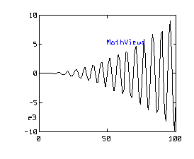
|
Related Topics:
Synopsis:
title(expr)
Description:
The title function outputs a text string at the top of the current graphics window.
Example:
|
INPUT |
OUTPUT |
| n=8
x=(0:n)/n y=x.*(1.2-x) y /= max(y) plot(x,y) title('title') |
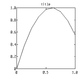
|
Related Topics:
Synopsis:
trace(expr)
Description:
The trace function returns the trace of its argument.
The function is defined for real and complex arrays. Scalar arguments are left unchanged by this function.
The trace of a matrix is defined as the sum of the diagonal elements of the matrix.
Example:
|
INPUT |
OUTPUT |
| A =
1 2 3 4 2 3 4 5 3 4 5 6 4 5 6 7 trace(A) |
ans =
16 |
Related Topics:
Synopsis:
tril(A)
tril(A, level)
Description:
The tril function returns the lower triangular matrix of A.
If the argument level is specified, then level > 0 includes up to the n-th level diagonal above the main diagonal. If level < 0, then the lower triangular matrix includes only up to the n-th level diagonal below the main diagonal.
If level equals 0, then the resulting matrix includes all elements up to the main diagonal.
Example:
|
INPUT |
OUTPUT |
| A =
1 2 3 4 2 3 4 5 3 4 5 6 4 5 6 7 tril(A) |
ans =
1 0 0 0 2 3 0 0 3 4 5 0 4 5 6 7 |
| tril(A,-1) |
ans = 0 0 0 0 2 0 0 0 3 4 0 0 4 5 6 0 |
| tril(A,2) |
ans = 1 2 3 0 2 3 4 5 3 4 5 6 4 5 6 7 |
Related Topics:
Synopsis:
triu(A)
triu(A, level)
Description:
The triu function returns the upper triangular matrix of A.
If the argument, level, is specified, then level > 0 includes up to the n-th level diagonal above the main diagonal. If level < 0, then the lower triangular matrix includes only up to the n-th level diagonal below the main diagonal.
If level equals 0, the resulting matrix includes all elements up to the main diagonal.
Example:
|
INPUT |
OUTPUT |
| A =
1 2 3 4 2 3 4 5 3 4 5 6 4 5 6 7 triu(A) |
ans =
1 2 3 4 0 3 4 5 0 0 5 6 0 0 0 7 |
| triu(A,1) |
ans = 0 2 3 4 0 0 4 5 0 0 0 6 0 0 0 0 |
Related Topics:
Synopsis:
type (filename)
Description:
The type command displays the contents of the named file.
Example:
type temp.tmp Displays the contents of the file, temp.tmp.
Related Topics:
Synopsis:
wbartlet(n)
Description:
The wbartlet function creates an n-point Bartlet window function
Example:
|
INPUT |
OUTPUT |
| wbartlet(9)' |
ans =
0 0.25 0.5 0.75 1 0.75 0.5 0.25 0 |
| plot(wbartlet(100)) |
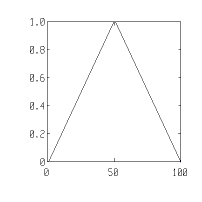
|
Related Topics:
wmerit, wrect, wsina, blackman, hamming, hanning
Synopsis:
who
whos
Description:
The who command lists the current variables in MathViews' memory.
The whos command also lists the current variables in MathViews' memory in addition to information about size, type of each variable.
Example:
who
whos
Related Topics:
Synopsis:
[pg, cg, enbw, sl, wcpl] = wmerit(win)
Description:
The wmerit function computes the figures of merit for the window function. These include processing gain, coherent gain, equivalent noise bandwidth, scalloping/picket fence loss, and worst-case processing loss.
The function parameters are:
|
pg |
processing gain |
| cg |
coherent (voltage) gain (normalized to the wrect(n)
window) |
| enbw |
equivalent noise bandwidth |
| sl |
scalloping loss or picket-fence loss (power) |
| wcpl |
worst case processing loss |
| win |
window function |
See F. J. Harris, On the Use of Windows for Harmonic Analysis with the Discrete Fourier Transform, in Proceedings of the IEEE, Vol. 66, No. 1, Jan 1978
Example:
|
INPUT |
OUTPUT |
| [pg,cg,enbw,sl,wcpl]=...
wmerit(blackman(64)); [pg cg enbw sl wcpl] |
ans =
0.5701 0.4139 1.754 0.8847 0.6679 |
| [pg,cg,enbw,sl,wcpl]=...
wmerit(hamming(64)); [pg cg enbw sl wcpl] |
ans =
0.6919 0.5128 1.445 0.8363 0.6957 |
| [pg,cg,enbw,sl,wcpl]=...
wmerit(hanning(64)); [pg cg enbw sl wcpl] |
ans =
0.6562 0.4925 1.524 0.8532 0.6912 |
Related Topics:
blackman, hamming, hanning, wbartlet, wrect, wsina
Synopsis:
wrect(n)
Description:
The wrect function creates an n-point rectangle window function. It is identical to ones(n,1).
Example:
|
INPUT |
OUTPUT |
| wrect(9)' |
ans =
1 1 1 1 1 1 1 1 1 |
Related Topics:
wmerit, blackman, hamming, hanning, wbartlet, wsina, ones
Synopsis:
wsina(n, p, woff)
Description:
The wsina function creates a family of sine windowing functions.
![]() k
= 0,1,2,, n1
k
= 0,1,2,, n1
The input parameters are:
|
n |
number of points |
| p |
power to which sin is raised (default = 1) |
| woff |
window bias (default = 0) |
The hamming and hanning functions are special cases of the wsina function.
Common values for p are 1, 2, 3, and 4.
Example:
See hanning.m and hamming.m M-files.
Related Topics:
hamming, hanning, wmerit, blackman, wbartlet, wrect
Synopsis:
x01(n)
Description:
The x01 function returns an n-point vector spaced linearly from 0 to 1.
Example:
|
INPUT |
OUTPUT |
| x01(6) |
ans =
0 0.2 0.4 0.6 0.8 1 |
Related Topics:
Synopsis:
x101(n)
Description:
The x101 function returns an n-point vector spaced linearly from -1 to 1.
Example:
|
INPUT |
OUTPUT |
| x101(6) |
ans =
-1 -0.6 -0.2 0.2 0.6 1 |
Related Topics:
Synopsis:
xlabel(expr)
ylabel(expr)
zlable(expr)
Description:
Each of these axis labeling functions outputs a text string next to the appropriate axis on the current graphics window in focus.
Example:
|
INPUT |
OUTPUT |
| n=8
x=(0:n)/n y=x.*(1.2-x) y /= max(y) plot(x,y) xlabel('x axis') ylabel('y axis') |
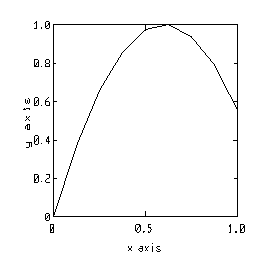
|
Related Topics:
Synopsis:
zeros(expr)
zeros(expr1, expr2)
Description:
The zeros function returns an array whose elements are 0's.
If the argument(s) is(are) integers, the function returns an expr by expr matrix (expr1 by expr2 matrix).
If the argument is an array, the result is an array with the same dimensions as the argument. The function returns a matrix with 0's as elements.
Example:
|
INPUT |
OUTPUT |
| zeros(3,4) |
ans =
0 0 0 0 0 0 0 0 0 0 0 0 |
| zeros(1) |
ans =
0 |
Related Topics:
Synopsis: _compile filename Description: The _compile (underscore compile) function compiles the file named filename. The M-file can either be a script M-file or a function M-file (see definitions section for description of file types). If filename is a function M-file, MathViews will insert the function into memory for faster subsequent accesses. Once the M-file is brought into memory, it stays there until the user clears the M-file from memory using the clear command, or the user exits MathViews. Script M-files are not retained in memory. The file, filename, does not have to be in single quotes or have a '.m' extension. The _compile function can also be invoked from the Program menu option (see user interface section). Example: _compile median _compile mesh
Synopsis:
_debug
Description:
The _debug command causes the program execution to halt as if a breakpoint had been set.
Example:
_debug Halt program execution at the current line.
Related Topics:
none
Synopsis:
_help
Description:
The help command displays all the underscore functions currently stored in memory.
Example:
|
INPUT |
OUTPUT |
| _help |
MathViews will display a list of all the
underscore functions. |
Related Topics:
Synopsis: _lcompile filename Description: The _lcompile (underscore l compile) function compiles the file, filename, and puts it into the MathViews memory. The file must be an L-file (library file). L-files are files that contain only functions. One can think of an L-file as a module containing many M-file functions (see definitions section for description of file types). Once the L-file is brought into memory, it stays there until the user clears the memory using the clear command or the user exits MathViews. When the L-file is in memory, all the functions in the L-file are available to the user. When a function in an L-file is invoked and the library file is not loaded into memory, MathViews will not recognize the function and will issue an error message. However, MathViews will search for M-files functions in the search path. The file, filename, does not have to be in single quotes or have a '.l' extension. L-files are loaded into memory through the compilation process. Example: _lcompile testmath
Synopsis: _list(type,name) Description: The _list function lists the available user-callable internal function, status in MathViews, and information in DLL and library files. The type argument must be an integer ( 0 or greater). _list(0) lists the current list of AutoAssign dependence variables in memory. _list(1) lists the DLL libraries which are currently loaded by MathViews. _list (1,'dllname') lists the imported functions in the specified DLL library. _list(2,'libname') lists all the functions which can be imported from the specified library name. Example: _list(0)
Synopsis: _loadlib libname Description: The _loadlib function loads a MathViews library file from the current working directory or the path specified by _MVPATH. Executing the _loadlib function will load the file mathview.mlb library file if no explicit name is specified. The library file must have been saved using the _savelib function. Example: _loadlib
Related Topics: _savelib
Synopsis: _savelib libname Description: The _savelib function saves the current contents of MathViews memory to the specified file. MathViews uses the name mathview.mlb if no specific file name is specified. The file is placed in the current working directory. Example: _savelib clear _loadlib
Related Topics: _loadlib
Synopsis: _ver Description: The _ver function shows the current version of MathViews. Example: _ver
The read/write variable _MVPATH stores the current search path. On powerup, _MVPATH is initialized from the MVPATH environment variable. The current working directory is also searched for unresolved m-files.
The read-only variable _MVPWD stores the current working dir.