![]()
![]()
![]()
![]()
![]()
Operations in the MathViews environment are based on statements. Statements are of the form:
variable = expression
or
expression
An expression is a sequence of operators, operands and punctuators that specifies a computation. Expressions are used to assign values to variables and to carry out a specific computation. MathViews uses the internal variable 'ans' if a variable is not given.
The principal data type in MathViews is a matrix of either real or complex values. Matrices of a single row or column can be thought of as vectors. MathViews has a number of functions and operators that manipulate matrices or vectors. You can also manipulate matrices and vectors on an element by element basis.
Results of computations are kept in variables. As in most programming languages, a variable occupies memory space and stores a value assigned to it. Assigning a value to a variable also specifies its type. For example,
| x = 2 x = 2 |
| sq = sin(x)^2 + cos(x)^2 sq = 1 |
MathViews automatically displays the result of evaluating the expression in the Output window. You can suppress the display in the Output window by placing a semicolon at the end of each assignment statement. For example,
| angle = cos(3*pi); |
Multiple assignment statements can be placed on a line by using the semicolon between statements. For example,
x = 2; sq = sin(x)^2 + cos(x)^2;
A MathViews variable can also be an ASCII string. An ASCII string must be enclosed in single quotation marks. Text strings are assigned in the following manner:
str = 'MathViews is Powerful';
Complex variables store complex (real and imaginary parts) rather than real numbers. The individual parts of a complex variable can be extracted using the real(z) and imag(z) MathViews functions. A complex variable can be assigned in one of the following ways:
| z = 2 + 4j
z = 2 + 4i z = 2 + i * 4 z = 2 + 4 * sqrt(-1) |
| eio = cos(2) + i * sin(2)
exp(2i) |
You can use either i or j to specify complex values. MathViews uses j to represent the imaginary part when it prints complex values. The multiplication symbol "*" is not required if the i or j is used after the real number representing the imaginary part. If the i or j is used ahead of the real number the multiplication symbol must be entered.
| z = 2 + 4j; |
| Valid assignment statement. |
| z = 2 + j4; |
| Invalid assignment statement, must use "*". |
Values in radians and degrees are also expressed in terms of complex numbers.
Vectors and Matrices can be thought of as arrays of values. Vectors are matrices with either one row or one column. From here on, the terms vector and matrix will be used interchangeably except where the distinction is meaningful. Matrices can have elements that are either complex or real. A matrix is considered to be complex if any element of the matrix is complex. A MathViews matrix can be entered in the following manner:
| A = [ 2 3 1; 4 3 2; 5 2 1] |
| A =
2 3 1 4 3 2 5 2 1 |
| A = [sqrt(-1) cos(0) sin(pi/2); exp(3) 2^2 5i] |
| A =
1j 1 1 20.0855 4 5j |
Row elements can either be separated by a comma or spaces. A semicolon is used to separate rows. Matrix assignments must be enclosed in square brackets, '[' ']'. Elements of a matrix can be accessed using the format A(index), where index begins at one. Elements are indexed in a column-wise fashion. For example,
| A =
2 3 1 4 3 2 5 2 1 |
| A(4) |
| ans =
3 |
| A(3) |
| ans =
5 |
| A(2) |
| ans =
4 |
You can also assign values to matrix elements that have not yet been allocated. For example,
| x = [ 2 3 1 ] |
| x =
2 3 1 |
| x(5) = 4 |
| x =
2 3 1 0 4 |
Assigning a value to the nonexistent fifth element in the x array causes an automatic expansion of the matrix to five elements and assignment of zero to the fourth element. The variable x must first exist for the assignment to be performed successfully.
MathViews makes a distinction between performing matrix type operations on a matrix and operating on a matrix on an element-by-element basis. The term array is used to refer to a matrix on which elemental operations are performed. Operations on matrices are performed with the matrices as a whole, whereas operations on arrays are performed on an element-by-element basis.
Transpose. MathViews uses the ' (apostrophe) character to denote transposition. An example will best explain the operator's function: Let
| A =
2 3 1 4 3 2 5 2 1 |
x =
1 2 3 4 |
Then
| x' |
| ans =
1 2 3 4 |
| A' |
| ans =
2 4 5 3 3 2 1 2 1 |
Addition and Subtraction. Both addition and subtraction are performed on an element by element basis. The dimension of both operands must be equal, except in the case where one is a scalar. MathViews will generate an error message if incompatible operands are used. For example,
| x=(x' + 5)' |
| x =
6 7 8 9 |
| A + A |
| ans =
4 6 2 8 6 4 10 4 2 |
| A= [ 1 2 3; 1 2 3] + [3 4; 2 3] |
|
Matrix Multiplication and Division. Matrix multiplication requires that the second dimension of the first operand be the same as the first dimension of the second operand. For example, if the first operand is m x 3, then the second operand must be 3 x n, and the resultant matrix will have dimensions of m x n. The relationship among the numbers of columns and rows of the operands and resultant matrix is as follows:
A * B = C
mxn nxp mxp
For example,
| A =
3 -1 4 2 0 1
|
B =
1 0 -3 -2 -2 4 5 -1 3 -1 0 6 |
| A * B |
| ans =
17 -8 -14 19 5 -1 -6 2 |
MathViews provides two matrix division operators, / and \. These correspond to right-hand and left-hand division, respectively. Matrix divisions follow the general rule: A/B is equivalent to A*inv(B) A\B is equivalent to inv(A)*B Array Multiplication and Division. MathViews performs array multiplication and division on an element by element basis. Array multiplication and division are denoted by placing a period (.) ahead of the *, /, and \ operators. Array multiplication and division are performed as follows: C = A.*B is equivalent to Ci = Ai * Bi C = A./B is equivalent to Ci = Ai/ Bi C = A.\B is equivalent to Ci = Bi / Ai For example,
| A =
2 3 1 4 3 2 5 2 1 |
| A .* A |
| ans =
4 9 1 16 9 4 25 4 1 |
| A ./ A |
| ans =
1 1 1 1 1 1 1 1 1 |
MathViews offers many methods for manipulating the data elements of a matrix. We will explore some of the more fundamental procedures for manipulating matrix elements in this section. The best way for learning how to manipulate matrices is to simply experiment with the operations discussed here. Colon Operator. The colon operator, ':', plays a very important role in matrix manipulation. Its simplest function is to assign a range of elements to a variable. For example,
| A = [ 1:4; 2:5 ] |
| A =
1 2 3 4 2 3 4 5 |
The general form of the colon operator is start:increment:end, corresponding to a starting value, an increment, and an ending value. The increment is assumed to be 1 if it is not explicitly specified. The colon operator is a simple way to generate a row vector covering a specified range of values.
| x = 0.5:0.5:2 |
| x =
0.5 1 1.5 2 |
Notice square brackets are not necessary when creating vectors using the colon operator.
| x = 2:-0.5:0.5 |
| x =
2 1.5 1 0.5 |
Negative numbers are also allowed for the increment value.
| x = sqrt(1:4) |
| x =
1 1.41421 1.73205 2 |
The colon operator can also be used to pass a range of values to a function.
| 1 + 1:5 |
| ans =
2 3 4 5 |
| 1 + (1:5) |
| ans =
2 3 4 5 6 |
The precedence of operators must be taken into consideration when creating expressions. Notice here the + operator has higher precedence than the colon operator. Care must be used when multiple operators are involved. Creating Matrices. Large matrices can be easily created using a combination of vectors and the colon operator. For example,
| x = [ 1 2 3]
x = [ x, 4 5 6] |
| x =
1 2 3 4 5 6 |
| A = [ x; 5:10] |
| A =
1 2 3 4 5 6 5 6 7 8 9 10 |
Matrix Subscripting: Matrix subscripting allows you to get access to individual matrix elements. The general form is as follows: A( rV, cV) The rV and cV arguments are subscripts and can be either scalars or vectors. When using subscripting you must ensure that the A matrix exists and that the ranges of the subscripts are subsets of the ranges of A. The elements of rV can not have values greater than the number of row of A and the elements of cV can not have values greater than the number of columns of A. The MathViews exist() function can be used to test for the existence of a variable. If the subscript variable is a vector, then only those elements of the matrix whose indices correspond to the values in the vector are accessed. This method is best illustrated by examples:
A =
1 2 3 4 5 6 7 8 9
1 2 3 4 5 6 7 8 9
1 2 3 4 5 6 7 8 9
1 2 3 4 5 6 7 8 9
1 2 3 4 5 6 7 8 9
1 2 3 4 5 6 7 8 9
1 2 3 4 5 6 7 8 9
1 2 3 4 5 6 7 8 9
1 2 3 4 5 6 7 8 9
| A(1:4, 1:4) |
| ans =
1 2 3 4 1 2 3 4 1 2 3 4 1 2 3 4 |
| A(3,:) |
| ans =
1 2 3 4 5 6 7 8 9 |
In the previous example, the colon operator was used with no values to select the third row of matrix A. Using the colon operator by itself corresponds to selecting all elements of the specified row or column. The third column of A could have been accessed by simply swapping the 3 and the :, i.e. A(:,3).
| x = [ 2 4 6]
A(:, x) = A(:,6:8) |
| A =
1 6 3 7 5 8 7 8 9 1 6 3 7 5 8 7 8 9 1 6 3 7 5 8 7 8 9 1 6 3 7 5 8 7 8 9 1 6 3 7 5 8 7 8 9 1 6 3 7 5 8 7 8 9 1 6 3 7 5 8 7 8 9 1 6 3 7 5 8 7 8 9 1 6 3 7 5 8 7 8 9 |
The columns 2, 4, and 6 of A are replaced by columns 6, 7, and 8 of A respectively.
| A(:,2:3) = A(:, 3:-1:2) |
| A =
1 3 6 7 5 8 7 8 9 1 3 6 7 5 8 7 8 9 1 3 6 7 5 8 7 8 9 1 3 6 7 5 8 7 8 9 1 3 6 7 5 8 7 8 9 1 3 6 7 5 8 7 8 9 1 3 6 7 5 8 7 8 9 1 3 6 7 5 8 7 8 9 1 3 6 7 5 8 7 8 9 |
This example switches columns 2 and 3.
| A(2:3, [1 1 2 2]) |
| ans =
1 1 3 3 1 1 3 3 |
This example selects from row 2 and 3, the first column twice and the second column twice. Matrix Reshaping: The colon operator can also be used on the left-hand side of an assignment statement to change the dimensioning or size of the matrix. For example,
| B =
1 2 3 2 3 4 |
| B(:) |
| ans =
1 2 2 3 3 4 |
This example changes the dimensions of B from a 2-by-3 matrix to a column vector whose elements are the columns of the previous B matrix.
| B(:) = 21:26 |
| B =
21 23 25 22 24 26 |
This example changes the values of the B matrix to the elements of a vector with values from 21 to 26. Notice that B retains its previous dimensioning.
| B(:) = [ 21 24 26 3 4 5] |
| B =
21 26 4 24 3 5 |
This example changes the values of the B matrix to the elements of the specified vector.
The matrix must already exist prior to using the colon operator to reshape matrices. The matrix must exist to maintain the same size, otherwise MathViews will create a column vector.
Matrix Shifting. Columns and rows of a matrix can be shifted to the left and right. Shifting can be either circular or linear. In a circular shift, as elements are shifted off the end they are wrapped back to the beginning. In a linear shift, as elements are pushed off the end, a zero value is added in place of the missing element. Here are some examples of performing linear and circular shifts:
| A =
1 2 3 4 5 6 7 8 9 10 11 12 13 14 15 16 |
| A >> [ 2 -2] |
| ans =
0 0 0 0 0 0 0 0 3 4 0 0 7 8 0 0 |
This example shows a linear shift of A by two elements down and two elements right. Notice that MathViews zero fills the remainder of A.
| A <> [ 2 -2] |
| ans =
11 12 9 10 15 16 13 14 3 4 1 2 7 8 5 6 |
In this example we perform a linear shift on the A matrix. Notice that in the circular case the elements that were shifted off are wrapped back around. The row shifts occur first, then the column shifts are performed. Deleting Matrix Rows/Columns. You can use the empty matrix notation, A = [] to easily delete matrix elements, columns, or rows. The empty matrix A is defined as a 0-by-0 matrix. A column or row is deleted in the following manner:
A =
1 2 3 4 5 6 7 8 9
1 2 3 4 5 6 7 8 9
1 2 3 4 5 6 7 8 9
1 2 3 4 5 6 7 8 9
| A(:, [ 1 3 5]) = [ ] |
| A =
2 4 6 7 8 9 2 4 6 7 8 9 2 4 6 7 8 9 2 4 6 7 8 9 |
This statement deletes column 1, 3, and 5.
| A([2 4],:) = [ ] |
| A =
2 4 6 7 8 9 2 4 6 7 8 9 |
This statement deletes rows 2 and 4. Logical Vectors. Matrices and vectors can be manipulated and reshaped using logical vectors. Logical vectors are vectors whose elements are either zero or one. A logical vector must have the same number of elements as the rows or columns they are referencing. The following examples illustrate the use of logical vectors:
| A =
1 2 3 4 5 6 7 8 9 10 11 12 x = 1 0 1 0 y = 0 1 0 |
Notice that the matrix A has three rows and four columns. The vector y has three elements and will be used to access the rows of matrix A. The vector x has four elements and will be used to access the columns of A.
| A(y,x) |
| ans =
5 7 |
The resultant matrix is those rows and columns of A for which the logical vectors, x and y, have a value of one.
| x =
1 1 1 1 y = 0 1 0 |
| A(y,x) |
| ans =
5 6 7 8 |
In this case the entire second row of A is returned since the logical vector y is all ones and the logical vector x has a one only in the second position.
| x =
1 1 1 |
| A(:,x) |
| ans =
1 1 1 5 5 5 9 9 9 |
In this example x is not treated as a logical vector for selecting columns from A since the number of elements of x is not equal to the number of columns of A. In this case, vector x is used as a subscript to select column one of A three times.
MathViews provides the pipe operator (->) to make the task of writing nested statements easier. The pipe operator allows you to send the output from one function into another function. This can eliminate the need for lots of parentheses and reduces the likelihood of making errors due too improper matching of parenthesis. For example,
| x =
1 2 3 |
| abs( sqrt( cos( exp(x)))) |
This expression can be converted into a simpler form with more readability using the pipe operator,
| exp(x)->cos->sqrt->abs |
| ans =
0.954848 0.669594 0.573232 |
MathViews provides a powerful facility for allowing you to set up automatic recalculations by assigning dependencies between variables. With the MathViews Auto-AssignTM technology you use the dependence assignment operator, :=, to build relationships among variables. Relationships can be nested many levels deep. MathViews will automatically update all dependent variables. For example,
| x = 1
y = 1 z = 2 |
| A := abs(x + y) |
| A =
2 |
This statement sets up the relationship that A is dependent on the value of the variables x and y.
| B := sqrt(z + A) |
| B =
2 |
This statement sets up the relationship that B is dependent on the value of variables z and A. B is indirectly dependent on the variables x and y since A is also dependent on the value of variables x and y.
| _list(0) |
| Your relations are :
Level 1 : A := x , y Level 2 : B := A , z |
The MathViews function _list() can be used to display the relationships you have set up.
| x = 4 |
| x =
4 A = 5 B = 2.64575 Variable Changed :B = 2.64575 Variable Changed :A = 5 |
Changing the value of x to 4 results in an automatic recalculation of the variables A and B. Recall that A is directly dependent on x and that B is indirectly dependent on x. Notice that all the appropriate related lower levels are updated before higher levels are updated. Auto-AssignTM technology and the dependent operator easily allow you to set up what-if type calculations. You can immediately see the effect changing a single value has on a set of equations.
Operating in the highly graphical Windows environment, MathViews offers a number of functions for generating high-quality graphic displays of your data. MathViews graph types include various x-y plots, polar plots, contour plots, and three-dimensional plots. The set of plotting functions in MathViews includes:
P
|
|
|
|
|
|
|
|
|
|
|
|
|
|
|
|
A number of functions are available for annotating the graphs once they are created. These include functions for titling, axis labeling, annotation text, and grids. The following functions are available in MathViews for annotating graphs:
A
|
|
|
|
|
|
|
|
|
|
|
|
|
|
MathViews also includes a number of additional functions for manipulating and printing graphics. The following additional graphics functions are provided:
G
|
|
|
|
|
|
|
|
|
|
|
|
|
|
|
The plot() function is the primary means of creating x-y plots in MathViews. In its simplest form, if plot is called with a vector, it automatically plots the data in a graphics window. MathViews automatically scales the plot to match the range of data. If plot is called with two vectors, it uses the first vector for the x-axis and the second vector for the y-axis. The following plot shows this case:
| t = 1:64
plot(t, sin(2*t/pi)) |
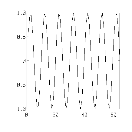
|
Multiple lines can be plotted on one graph by using multiple arguments to the plot() function. You can also specify line style, symbol type and color. The following example plots two lines on the same graph window. The first line is plotted in green and uses the + symbol and the second line is plotted in red and uses the * symbol. Notice also that we use the hold function to hold the plot while we redraw the lines using solid lines with no symbols.
| t = 0:32
t2 =-400 + t^2; t4 = 4*t.*sin(t); plot(t,t2,'+g', t, t4, '*r') hold on plot(t,t2,t,t4) hold off |
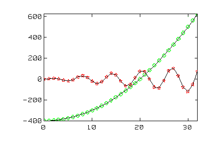 |
Other MathViews functions can be used to generate x-y plots with different x-y axis scaling. The loglog(), semilogx(), and semilogy() functions allow you to generate various logarithmic scaling.
The polar() function is used to create polar plots in MathViews. This function takes two arguments, the first specifies the angle and the second specifies the length of the vector at the corresponding angles. The following example shows how to create a polar plot. Notice again the use of the hold function to allow multiple plots to be place into one graphics window. The grid function places a polar grid on the window.
| pi = acos(-1);
theta=0:.1:4*pi; r=4+4*sin(theta); r1=3+5*sin(theta); r2 = 6+4*sin(theta); polar(theta,r2); hold on polar(theta,r1); polar(theta,r); grid |
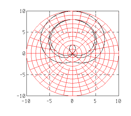 |
The contour() function is used to create contour plots in MathViews. In its simplest form, this function takes a 2-dimensional array of real values and creates a contour with 10 levels. The following example shows this case:
| n=8;
x=(0:n)/n; y=x.*(1.2-x); y /= max(y); z=y'*y; contour(z) |
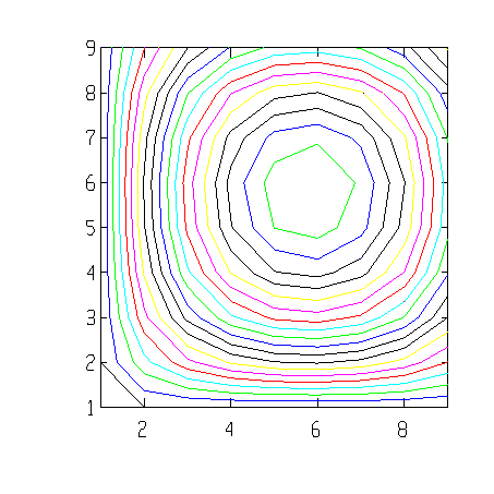 |
Additional arguments to the contour function allow you to specify the number of levels or the specific levels at which you wish to plot contours.
The mesh() function is used to create three-dimensional plots in MathViews. In its simplest form, this function takes a two-dimensional array of real values that indicates the height, Z-axis value, above the X-Y plane. The following example illustrates this case:
| n=8;
x=(0:n)/n; y=x.*(1.2-x); y /= max(y); z=y'*y; mesh(z) |
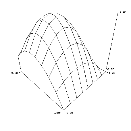 |
Additional parameters to the mesh function allow you to change the viewing angle and distance.
Relational and logical operators are used to test the validity of two expressions based on a specified relationship. They operate on matrices on an element-by-element basis. The results of both relational and logical operations are 0 or 1.
The set of relational operators in MathViews includes:
R
|
|
|
|
|
|
|
|
|
|
|
|
|
|
A MathViews relation has the form: { expr } ( relational operator) { expr } The relational operator is applied to the matrices resulting from the expressions on an element-by-element basis. The resultant matrices must be of equal dimensions. The resultant value is a 1 if the relationship holds; otherwise it is a 0. For example,
| A =
1 2 3 4 5 6 7 8 9 10 11 12 |
B =
9 2 45 4 4 6 8 8 9 20 11 12 |
| x = (A >= 5) |
| x =
0 0 0 0 1 1 1 1 1 1 1 1 |
This relationship returns matrix x with a one for each element of matrix A that has a value greater than or equal to 5.
| x = A == B |
| x =
0 1 0 1 0 1 0 1 1 0 1 1 |
This relationship returns a matrix x with a one for each element of matrix A that is also in matrix B.
The set of logical operators in MathViews includes:
|
|
|
|
|
|
A logical comparison has the form: { expr } ( logical operator) { expr } The result of logical operators is a 1 if the logical condition holds and a 0 if the logical condition fails. The binary logical operators (& and |) must have operands whose dimensions are equal. The not logical operator (~) is unary. Logical operators function on elements of matrices, usually with logical matrices. The following examples illustrate the concept:
| A =
1 0 1 0 1 0 |
B =
1 1 1 0 1 1 |
| A | B |
A & B |
| ans =
1 1 1 0 1 1 |
ans =
1 0 1 0 1 0 |
Like most programming languages, MathViews has statements to control the flow of execution of statements. Looping constructs, such as while and for loops, can be used to repeat a set of statements either until a condition is met or a set number of times. Conditional statements can be used to execute a set of statements based on specified conditions.
The if statement is used allow conditional execution, based on the evaluation of an expression. An if statement must terminate with the keyword end. The general form is as follows:
if expression
statements
end
or
if expression
statements
else[if expression]
statements
end
The expression evaluates to true if it has a value, or elements with value, greater or equal to 1; otherwise it is false. The else and elseif conditionals are optional. The condition expression resultant must be a scalar. The following examples illustrate the use of if statements:
| A =
1 0 1 0 1 0 B = 1 1 1 0 1 1 C = 1 1 1 0 1 1 |
| if ( all(all(A == B)))
disp('B equal to A') else disp('B not equal to A') end |
| B not equal to A |
| if ( all(all(C == A)))
disp('C is equal to A') elseif all(all(C == B)) disp('C is equal to B') end |
| C is equal to B |
The MathViews all() function is used to compare all elements of the matrix it is passed to see if they are greater than or equal to 1.
While Loops. The while construction executes a series of statements in a loop as long as a given condition is true. The general form is as follows:
while condition
statement
end
The condition is usually a scalar result of a relational operation. As with the if statement, you could use the all() function to obtain a scalar condition from a condition matrix. The following example illustrates the use of a while loop:
| x = 0
while( x < 5 ) disp(x++) end |
This example displays the numbers from 0 to 4. The while loop stops executing when the value of x is no longer less than five.
For Loops. The for loop repeats a group of instructions for a specified number of times. The general form is as follows:
for n = expression
statements
end
The for loop expression in MathViews is a matrix. The statements in the for loop get executed once for each column of the expression matrix. The for loop variable, n, is assigned the value of the current column of the expression matrix. The expression matrix is typically a vector created with the colon operator, i.e. for n = 1:5, would cause the statements to be executed five times, with n taking on the integer values from 1 to 5. The following example shows the use of nested for loops and the size() function. The size() function is used to determine the number of elements in a matrix. The matrix dimensions are used to specify the number of times to execute the statements in the for loop.
| A =
1 2 3 4 5 6 7 8 9 1 2 3 4 5 6 7 8 9 1 2 3 4 5 6 7 8 9 1 2 3 4 5 6 7 8 9 1 2 3 4 5 6 7 8 9 1 2 3 4 5 6 7 8 9 1 2 3 4 5 6 7 8 9 1 2 3 4 5 6 7 8 9 1 2 3 4 5 6 7 8 9 |
| [m, n] = size(A);
for i = 1:m for j = 1:n if ( i ~= j) A(i,j) = A(j,i); end end end A |
| A
ans = 1 1 1 1 1 1 1 1 1 1 2 2 2 2 2 2 2 2 1 2 3 3 3 3 3 3 3 1 2 3 4 4 4 4 4 4 1 2 3 4 5 5 5 5 5 1 2 3 4 5 6 6 6 6 1 2 3 4 5 6 7 7 7 1 2 3 4 5 6 7 8 8 1 2 3 4 5 6 7 8 9 |
The break statement is used to terminate from within an iteration statement. Break can be used in the body of while or for looping constructs. When used within nested looping constructs, break transfers control to the loop that is nested one level above the loop in which it occurs. For example,
| A =
1 1 1 1 1 1 1 1 1 1 2 2 2 2 2 2 2 2 1 2 3 3 3 3 3 3 3 1 2 3 4 4 4 4 4 4 1 2 3 4 5 5 5 5 5 1 2 3 4 5 6 6 6 6 1 2 3 4 5 6 7 7 7 1 2 3 4 5 6 7 8 8 1 2 3 4 5 6 7 8 9 |
| for i = 1:m
for j = 1:n A(i,j) = i * j; if ( (i == 2) & (j ==2)) break elseif ( (i == 4) & (j == 4)) break elseif( (i==6) & (j==6)) break end end end A |
| A
ans = 1 2 3 4 5 6 7 8 9 2 4 2 2 2 2 2 2 2 3 6 9 12 15 18 21 24 27 4 8 12 16 4 4 4 4 4 5 10 15 20 25 30 35 40 45 6 12 18 24 30 36 6 6 6 7 14 21 28 35 42 49 56 63 8 16 24 32 40 48 56 64 72 9 18 27 36 45 54 63 72 81 |
MathViews can be used in an interactive mode to provide solutions to your problems. However, MathViews can also be programmed to control repetitive tasks or to extend the MathViews language itself. MathViews, as was discussed in the previous section, provides statements that control the flow of execution of your statements.
MathViews programs are written in units called M-files. M-files are stored on the disk in files with extensions of ".M". There are two types of M-files:
Script M-files contain a set of statements that are executed when the script file is invoked.
Function M-files are similar to script files. In addition to containing a set of statements that are executed, they can also be passed parameters and return results. Only one function can be specified per M-file.
MathViews also supports another type of file that is extremely useful for maintaining your functions when developing a large project. L-files serve as modules that can contain multiple functions. This overcomes the limitation of only having one function per file as in M-files.
Script M-files contain sequences of statements. The script M-file is invoked by calling the name of the M-file. For example, suppose the following script is stored in the file maxval.m. This script file finds and prints the maximum value contained in the matrix A. Executing the script by entering maxval causes the maximum value in matrix A to be printed. The matrix A must exist prior to executing this M-file.
| %
% Script M-file to find the maximum value % in the matrix A. % [m,n] = size(A); max = -1e300; for x = 1:m for y = 1:n if A(x,y) > max max = A(x,y); end end end max |
Script files are executed as if you had entered them in interactive mode. Any variables created in the script file are left in the MathViews environment upon completion of the script.
Functions defined in a function M-file can be used to extend the MathViews language. Function files are similar to script files in that they both contain a set of statements to be executed, however, there are a few important differences. The first line of a function file must contain the word function. Functions can also be passed arguments and can return values. Also, unlike script M-files, variables created in a function M-file only exist during the execution of the function. They are not left in the MathViews environment upon completion of the function. Only one function can be defined per M-file. The following example performs the same operations as the script file discussed above, that is, finding the maximum value of a matrix. However, the function we create will be passed the matrix for which we wish to find the maximum and it will return the maximum value as a variable.
function max = maxval(a)
%
% Function M-file to find the maximum value
% in the matrix a.
%
[m,n] = size(a);
max = -1e300;
for x = 1:a
for y = 1:a
if a(x,y) > max
max = a(x,y);
end
end
end
The first line of the function M-file defines the input and output parameters for the function. There is one input variable, a, and one output variable, max. If we store this function in an M-file named maxval.m, we can invoke it using the form:
maximum = maxval(A)
In this case, we pass the matrix A as an argument to maxval. The maxval function M-file operates on the matrix A and returns the maximum value.
MathViews library module files overcome the limitations of only allowing a single function per M-file. A library module file, L-file, contains only functions in the form discussed above for function M-files. Functions can be grouped according to the specific application they were designed for. This simplifies management of the functions you create by placing all related functions into one location. MathViews lets you easily load a function library file into memory by executing the _lcompile statement.
MathViews provides a number of powerful debugging features to quickly let you get your programs up and running. Debugging features include the ability to set breakpoints, single step the program, view variables in a separate window, view the current call stack, and animate the operation of the program. Debugging features are accessed through the Debug menu item, or by using the right mouse button in the edit window.
MathViews allows you to set a breakpoint on any line of any M-file in your program. Program execution will halt when the breakpoint is reached. At that point, you can either examine the variables in your program, examine the program call stack, single-step the program, or continue execution. Breakpoints are set on the program window line containing the flashing text cursor by either of two methods. The first method is to display a popup menu using the right mouse button while the cursor is in the program window. This popup menu has entries for setting or resetting breakpoints. To set the breakpoint simply click on the Set menu item using the left mouse button. The second method of setting breakpoints is to use the Set Breakpoint menu item under the toplevel Debug menu. This entry can also be reached using the Ctrl-B key combination. The current set of breakpoints are listed in the Breakpoint window. The Breakpoint window entry lists the file name and the line number on which the breakpoint occurs. Breakpoints can be cleared using one of three methods. The first two are similar to those used for setting the breakpoints and operate on the line containing the text entry cursor in the program window. These two methods are using the Reset menu item on the popup menu accessed through the right mouse button in the program window or using the Reset Breakpoint menu item from the top level Debug menu. The Debug menu Reset Breakpoint menu item can be accessed using the Ctrl-N key combination. The third method of resetting breakpoints is to click on a breakpoint entry in the Breakpoint window using the left mouse button. MathViews will display a dialog box asking you if you wish to clear the breakpoint. Breakpoints are disabled by default. Breakpoints can be enabled using the Breakpoint Enabled menu item from the top level Debug menu. MathViews places a check mark next the Breakpoint Enabled menu item to indicate that breakpoints are enabled. The _debug command can be used to place a hard breakpoint into the program. The program is halted as if a user-specified breakpoint had been set at that program line.
MathViews lets you single-step through your program using either menu items or key strokes. The Step Over and Trace Into menu items from the top level Debug menu allow you to single step your program. These menu items can be accessed using the F8 and F7 keys respectively. The Step Over single step command will execute each line of your program but will not step into any functions. Instead, functions will be executed and program execution will continue to the next line of your program. The Trace Into command performs similar to the Step Over command, however, it will allow you to step into a function. Program execution continues on the first line of the M-file containing the function you traced into.
The current program call stack can be viewed in the Stack window. Information contained in the Stack windows includes the current function being executed, the Line at which the function was called, whether Trace is enabled, and the name of the file containing the function. The Stack window is updated as the program is executed. As you single-step through your program you can always see which function is being executed and which execution path was used to reach the function.
MathViews variables can be examined using the Variables window. The variables window shows the variables visible in the current function scope. In order to improve performance, the variables window is only updated whenever it is selected. The window is divided into two areas. The variables list on the left side of the window shows a list of the currently visible variables. The value of a variable can be examined by selecting it using the left mouse button. The value is displayed in the scrollable area in the right-hand side of the variables window.
A MathViews program can be automatically single-stepped using the Animate menu item from the top level Debug menu. This menu item can also be accessed using the F3 function key. The Animate command can also be issued after a breakpoint has been used to halt the program execution.
![]()
![]()
![]()
![]()
![]()