This case study demonstrates the application of
several techniques described in this paper to the quantitative
measurement of a peak that is buried in an unstable background,
a situation that can occur in the quantitative analysis
applications of various forms of spectroscopy, process
monitoring, and remote sensing. The objective is to derive a
measure of peak amplitude that varies linearly with the actual
peak amplitude but that is not effected by the changes in the
background and the random noise. In this example, the peak to be
measured is located at a fixed location in the center of the
recorded signal, at x=100 and has a fixed shape (Gaussian) and
width (30). The background, on the other hand, is highly
variable, both in amplitude and in shape. The simulation shows
six superimposed recordings of the signal with six different
peak amplitudes and with randomly varying background amplitudes
and shapes (top row left in the following figures). The methods
that are compared here include smoothing, differentiation,
classical
least squares multicomponent method (CLS), and iterative
non-linear curve fitting.
CaseStudyC.m is a
self-contained Matlab/Octave demo function that demonstrates
this case. To run
it, download it. place it in the path, and type "CaseStudyC" at
the command prompt. Each time you run it, you'll get the same
series of true peak amplitudes (set by the" vector
SignalAmplitudes", in line 12) but a different set of background
shapes and amplitudes. The background is modeled as a Gaussian
peak of randomly varying amplitude, position, and width; you can
control the average amplitude
of the background by changing the variable
"BackgroundAmplitude" and the average change
in the background by changing the variable
"BackgroundChange".
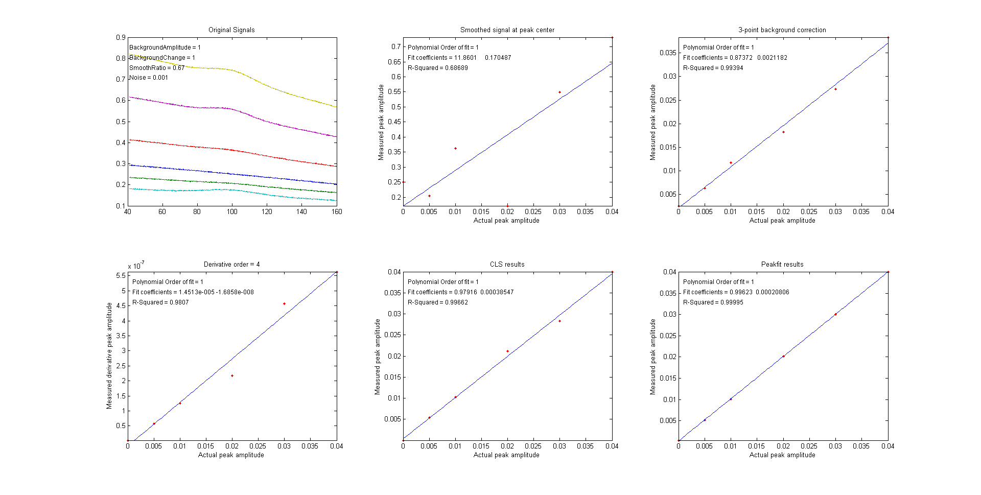
The five methods compared in the figures below are:
1: Top row center. A simple zero-to-peak measurement of the smoothed signal, which assumes that the background is zero.
2: Top row right. The difference between the peak signal and the average background on both sides of the peak (both smoothed), which assumes that the background is flat.
3: Bottom row left. A derivative-based method, which assumes that the background is very broad compared to the measured peak.
4: Bottom row center. Classical least squares (CLS), which assumes that the background is a peak of known shape, width, and position (the only unknown being the height).
5: Bottom row right. iterative non-linear curve fitting (INLS), which which assumes that the background is a peak of known shape but unknown width and position. This method can track changes in the background peak position and width (within limits), as long as the measured peak and the background shapes are independent of the concentration of the unknown.
These five methods are listed roughly in the order of increasing mathematical and geometrical complexity. They are compared below by plotting the actual peak heights (set by the vector "SignalAmplitudes") vs the measure derived from that method, fitting the data to a straight line, and computing the coefficient of determination, R2., which ideally is 1.0000.
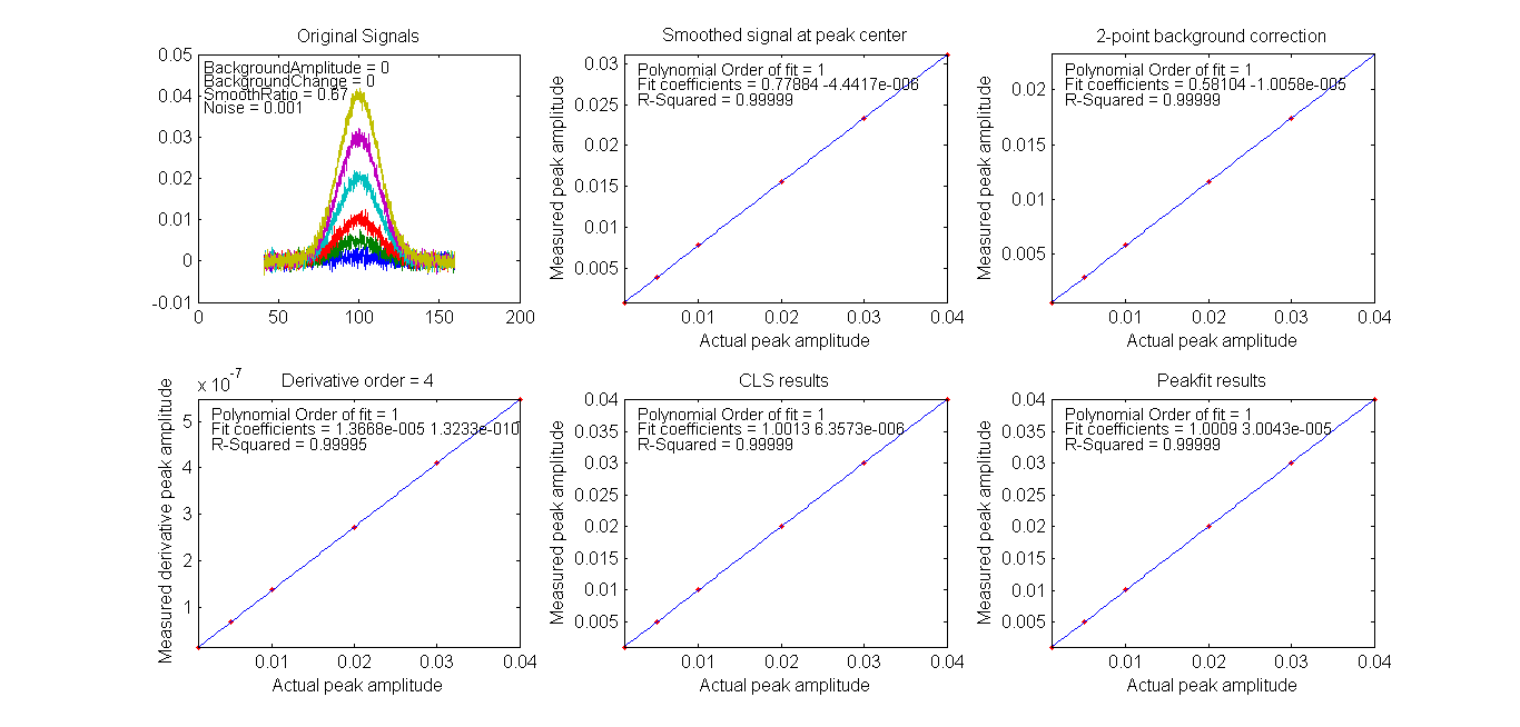
 For
the first test (shown in the figure above), both
"BackgroundAmplitude" and "BackgroundChange" are set to zero, so
that only the random noise is present. In that case all the
methods work well, with R2.values all very close to 0.9999. With a 10x higher
noise level (click
to view), all methods still work about equally well, but
with a lower coefficient of determination R2, as might be expected.
For
the first test (shown in the figure above), both
"BackgroundAmplitude" and "BackgroundChange" are set to zero, so
that only the random noise is present. In that case all the
methods work well, with R2.values all very close to 0.9999. With a 10x higher
noise level (click
to view), all methods still work about equally well, but
with a lower coefficient of determination R2, as might be expected.
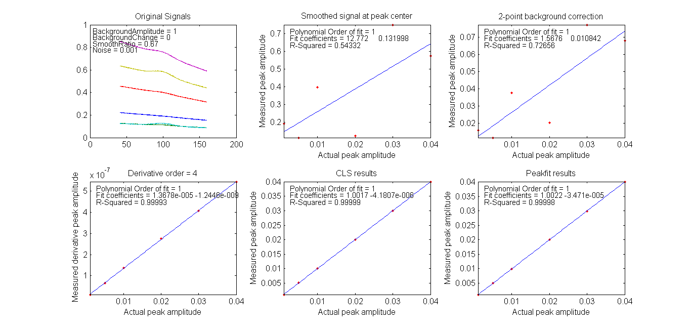
For the second test (shown in the figure immediately above), "BackgroundAmplitude"=1 and "BackgroundChange"=0, so the background has significant amplitude variation but a fixed shape, position, and width. In that case, the first two methods fail, but the derivative, CLS, and INLS methods work well.
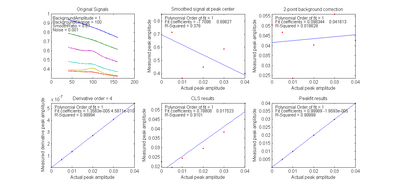
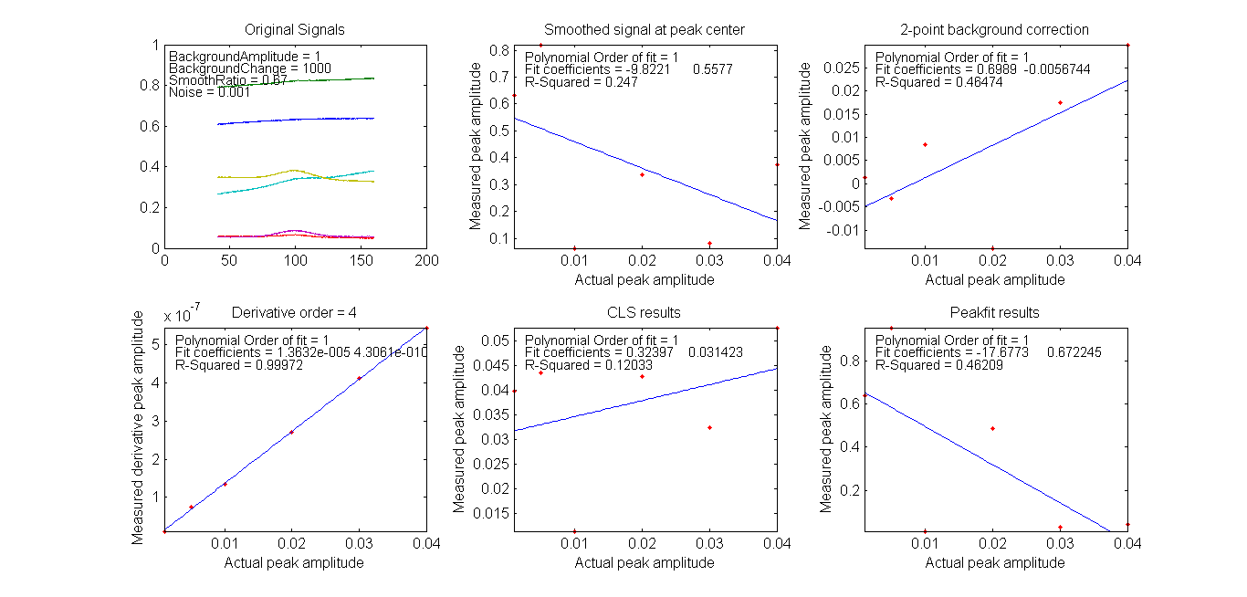
For the third test, shown in the figure above, "BackgroundAmplitude"=1 and "BackgroundChange"=100, so the background varies in position, width, and amplitude (but remains broad compared to the signal). In that case, the CLS methods fails as well, because it assumes that the background varies only in amplitude. However, if we go one step further (click to view) and set "BackgroundChange"=1000, the background shape is now so unstable that even the INLS method fails, but still the derivative method remains effective as long as the background is broader than the measured peak, no matter what its shape. On the other hand, if the width and position of the measured peak changes from sample to sample, the derivative method will fail and the INLS method is more effective (click to view), as long as the fundamental shape of both measured peak and the background are both known (e.g. Gaussian, Lorentzian ,etc).
Not surprisingly, the
more mathematically complex methods perform better, on average.
Fortunately, software can "hide" that complexity, in the same
way, for example, that a hand-held calculator hides the
complexity of long division.
This page is part of "A Pragmatic Introduction to Signal
Processing", created and maintained by Tom O'Haver, Professor
Emeritus, Department of Chemistry and Biochemistry, The University
of Maryland at College Park. Comments, suggestions and questions
should be directed to Prof. O'Haver at toh@umd.edu. Updated July, 2022.