B. Signal or Noise?

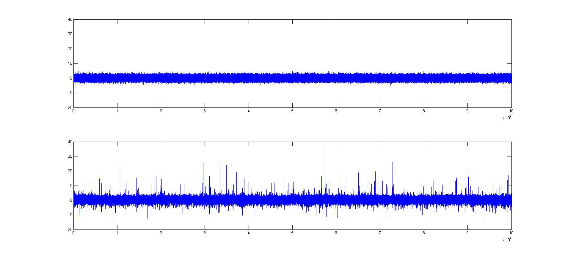
This experimental signal in this case study was unusual because it did not look like a typical signal when plotted; in fact, it looked a lot like noise at first glance. The figure below compares the raw signal (bottom) with the same number of points of normally-distributed white noise (top) with a mean of zero and a standard deviation of 1.0 (obtained from the Matlab/Octave 'randn' function).  

As you can see, the main difference is that the signal has more large 'spikes', especially in the positive direction.  This difference is evident when you look at the descriptive statistics of the signal and the randn function:

You can see that the standard deviations of these two are nearly the same, but the other statistics (especially the kurtosis and skewness) indicate that the probability distribution o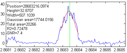f the signal is far from normal; there are far more positive spikes in the signal than expected for pure noise. Most of these turned out to be the peaks of interest for this signal; they look like spikes only because the length of the signal (over 1,000,000 points) causes the peaks to be compressed into one screen pixel or less when the entire signal is plotted on the screen. In the figures on the left, iSignal is used to "zoom in" on some of the larger of these peaks (using the cursor arrow keys). The peaks are very sparsely separated (by an average of 1000 half-widths between peaks) and are well above the level of background noise (which has a standard deviation of roughly 0.9 throughout the signal).

The researcher who obtained this signal said that a 'good' peak was 'bell shaped', with an amplitude above 5 and a width of 500-1000 x-axis units. So that means that we can expect the signal-to-background-noise ratio to be at least 5/0.9 = 5.5. You can see in the three example peaks on the left that the peak widths do indeed meet those expectations. The interval between adjacent x-axis points is 25, so that means the we can expect the peaks to have about 20 to 40 points in their widths. Based on t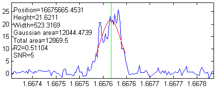hat, we can expect that the positions, heights and widths of the peaks should be able to be be measured fairly accurately using least-squares methods (which reduce the uncertainty of measured parameters by about the square root of the number of points used - about a factor of 5 in this case). However, the noise appears to be signal-dependent; the noise on the top of the peaks is distinctly greater than the noise on the baseline. The result is that the actual signal-to-noise (S/N) ratio of peak parameter measurement for the larger peaks will not be as good as might be expected based on the ratio of the peak height to the noise on the background.  Most likely, the total noise in this signal is the sum of two major components, one with a fixed standard deviation of 0.9 and the other roughly equal to 10% of the peak height.

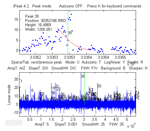
To automate the detection of large numbers of peaks, we can use the findpeaksG or iPeak functions. Reasonable values of the input arguments AmplitudeThreshold, SlopeThreshold, SmoothWidth, and FitWidth for those functions can be estimated based on the expected peak height (5) and width (20 to 40 data points) of the "good" peaks. For example, using 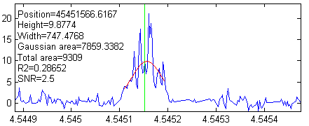AmplitudeThreshold=5, SlopeThreshold=.001,  SmoothWidth=25, and FitWidth=25, these function detect and measure 76 peaks above an amplitude of 5 and with an average peak width of 523. The interactive iPeak function is especially convenient for exploring the effect of these peak detection parameters and for graphically inspecting the peaks that it finds. Ideally the objective is to find a set of peak detection arguments that detect and accurately measure all the peaks that you would consider 'good' and skip all the 'bad' ones. But in reality the criteria for good and bad peaks is at least partly subjective, so it's usually best to err on the side of caution and avoid skipping 'good' peaks at the risk of including a few 'bad' peaks in the mix, which can be weeded out manually based on unusual position, height, width, or appearance.  

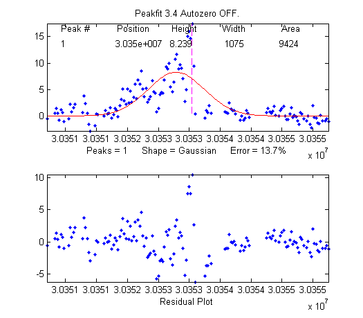
Of course, it must be expected that the values of the peak position, height, and width given by the findpeaksG or iPeak functions will only be approximate and will vary depending on the exact setting of the peak detection arguments; the noisier the data, the greater the uncertainty in the peak parameters. In this regard the peak-fitting functions peakfit.m and ipf.m usually give more accurate results, because they make use of all the data across the peak, not just the top of the peak as do findpeaksG and iPeak. For example, compare the results of the peak near x=3035200 measured with iPeak (click to view) and with peakfit (click to view). Also, the peak fitting functions are better for dealing with overlapping peaks and for estimating the uncertainty of the measured peak parameters, using the bootstrap options of those functions. For example, the largest peak in this signal has an x-axis position of 2.8683e+007, height of 32, and width of 500; the bootstrap method determines that the standard deviations are 4, 0.92,  and 9.3, respectively. 

Because the signal in the case study was so large (over 1,000,000 points), the interactive programs such as iPeak, iSignal, and ipf may be sluggish in operation, especially if your computer is not fast computationally or graphically. If this is a serious problem, it may be best to break the signal up into two or more segments and deal with each segment separately, then combine the results. Alternatively, you can use the condense function to average the entire signal into a smaller number of points by a factor of 2 or 3 (at the risk of slightly reducing peak heights and increasing peak widths), but then you should reduce SmoothWidth and FitWidth by the same factor to compensate for the reduced number of data points across the peaks.  Run testcondense.m for a demonstration of the condense function.