


The objective of this
exercise is to learn as much as we can about the underlying
properties of a digitized signal using the signal processing
tools in this book and, if possible, to obtain a mathematical
description of the signal (script).
At
first glance, the signal (MysteryPeak.mat) appears to be a single, asymmetrical peak
with a maximum at x=55.5. The signal-to-noise ratio seems to be
very good - there is little visible noise unless you look very
closely - and the signal begins and ends near zero, so baseline
correction is likely not an issue. The bad news is that we do
not know anything else. The asymmetry might be due to some
asymmetrical process applied to an originally symmetrical peak
shape, but it could be a group of closely spaced overlapping
peaks, which is suggested by the faint bumps in the shape. Some
quick preliminary curve fitting can be done using command line peakfit.m:
for a
two-Gaussian model (shape 1)
[FitResults,GOF]=peakfit([x
y],0,0,2,1)
for
a single Logistic model (shape 3)
[FitResults,GOF]=peakfit([x
y],0,0,1,3)
for a 4
exponentially broadened Gaussian model (shape 39)
[FitResults,GOF]=peakfit([x y],0,0,4,39,1)

Alternatively, it is even easier to use the interactive peak
fitter ipf.m for this
purpose; you can quickly change the model shape, number of
peaks, starting guesses, data region to be fitted, etc., with
single keystrokes and mouse clicks. Either way, the three
initial fits in the figures show that the signal contains a
small amount of random noise, which appears to be white (so the
signal has probably not been smoothed, which is fortunate) and
which has a relative standard deviation of about 0.2%, based on
1/5th of the visual peak-to-peak value in the
residual plot. But
unfortunately these fits are not successful because their
fitting errors (0.5 to 0.8%) are all significantly larger than
the 0.2% random noise. Trying different shapes and greater
numbers of peaks does not help either, resulting in either
higher fitting errors, unstable fits, or zero peak heights for
additional peaks (as in the four-Gaussian fit).
 Another approach
to the problem of asymmetrical peaks is to use the technique of
first-derivative
symmetrization described previously. This applies specifically to exponential
broadening, a commonly- encountered peak broadening mechanism. The
idea is that if you compute the first derivative of an
exponentially broadened peak, multiply it by a weighting factor
equal to the time constant of the exponential, and add it to the
original broadened signal, the result will be the original peak
before broadening, which makes the peak overlap less severe.
This works for any
original
peak shape. Even if you
do not know the time constant beforehand, you can try different
values until the baseline after the peak is as low as possible
but not negative, as shown in this
GIF
animation. This is easily
done interactively in iSignal, version 7, which has smoothing,
derivatives, symmetrization, and curve fitting, or by using the
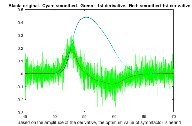
symmetrize.m function. The derivative of y with respect
to x, by the "derivxy.m" function, shown by the green line in the
figure above, is quite noisy. As usual, we must smooth the
derivatives of noisy signals to make them useful, but we must
not over-smooth and distort the signals. As a rule of thumb, a
smooth width equal to 1/10th of the number of data
points in the halfwidth does not distort the signal visibly.
  Our peak has about
530 points (=halfwidth(1:length(y),y)), so a smooth width near 53
will not distort the signal peak, but it does eliminate most of
the noise from the derivative (red line, above right). Also, we
can see that the derivative, in y/x units, is comparable in
numerical magnitude to the original signal, so the weighting
factor (in x units) is probably somewhere near 1.0. Next, we add
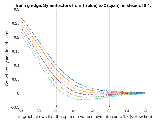
the first derivative times that factor to the original signal,
looking at the trailing edge as we try six different factor
values near 1.0. The graph on the left shows that the optimum
value is about 1.25.
When this symmetrization is applied to the
entire signal, the result, shown below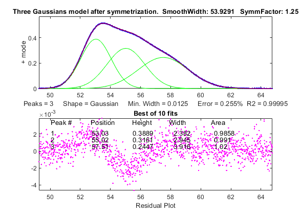 on the right, has
more distinct bumps. When that modified signal is used for curve
fitting, it is found that a 3-Gaussian model works quite well,
with a fitting error of only 0.25%. This is evidence that the
signal actually consists of three exponentially broadened
Gaussians. Ordinarily there is no independent way to check the
accuracy of the peak parameters so measured, but - full
disclosure - the signal in the case was not actually unknown but
rather was generated by the file MysteryPeaks.m. The true time constant is 1.3, the peak
positions are 53, 55, and 57.5 and the peak areas are each equal
to 1.0. The curve-fit results after symmetrization (shown
on the right) are within 0.1% for the peak positions and within
2% of the areas. In contrast, direct fitting of three
equal-alpha exponential Gaussians to the original data, which is
now possible because we have determined a value for the time
constant (expressed as the number of data points: symmfactor./(x(2)-x(1)), gives less accurate results
in this case (graphic), probably because the
overlap of the asymmetrical peak is greater. Moreover, it takes
three times longer to compute.
This page is part of "A Pragmatic Introduction to Signal
Processing", created and maintained by Tom O'Haver, Professor
Emeritus, Department of Chemistry and Biochemistry, The University
of Maryland at College Park. Comments, suggestions and questions
should be directed to Prof. O'Haver at toh@umd.edu. Updated July, 2022.

 Another approach
to the problem of asymmetrical peaks is to use the technique of
first-derivative
symmetrization described previously. This applies specifically to exponential
broadening, a commonly-
 Our peak has about
530 points (=halfwidth(1:length(y),y)), so a smooth width near 53
will not distort the signal peak, but it does eliminate most of
the noise from the derivative (red line, above right). Also, we
can see that the derivative, in y/x units, is comparable in
numerical magnitude to the original signal, so the weighting
factor (in x units) is probably somewhere near 1.0. Next, we add
the first derivative times that factor to the original signal,
looking at the trailing edge as we try six different factor
values near 1.0. The graph on the left shows that the optimum
value is about 1.25.
  on the right, has
more distinct bumps. When that modified signal is used for curve
fitting, it is found that a 3-Gaussian model works quite well,
with a fitting error of only 0.25%. This is evidence that the
signal actually consists of three exponentially broadened
Gaussians. Ordinarily there is no independent way to check the
accuracy of the peak parameters so measured, but - full
disclosure - the signal in the case was not actually unknown but
rather was generated by the file MysteryPeaks.m. The true time constant is 1.3, the peak
positions are 53, 55, and 57.5 and the peak areas are each equal
to 1.0. The curve-fit results after symmetrization (shown
on the right) are within 0.1% for the peak positions and within
2% of the areas. In contrast, direct fitting of three
equal-alpha exponential Gaussians to the original data, which is
now possible because we have determined a value for the time
constant (expressed as the number of data points: symmfactor./(x(2)-x(1)), gives less accurate results
in this case (graphic), probably because the
overlap of the asymmetrical peak is greater. Moreover, it takes
three times longer to compute.