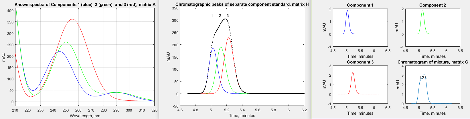
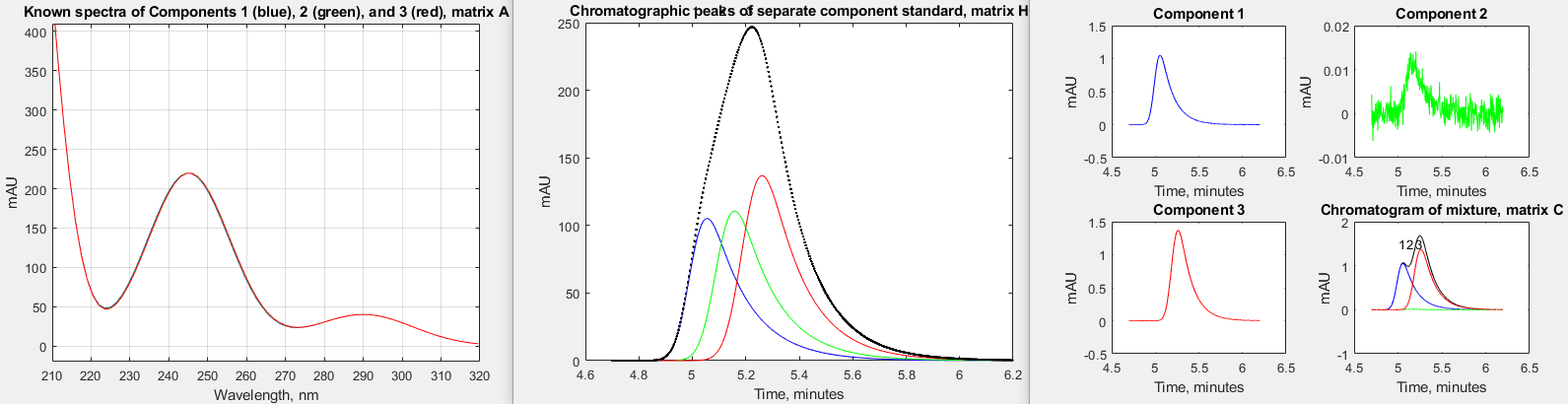
The introduction of high-speed UV-Visible array detectors into high performance liquid chromatography (HPLC) instruments has significantly increased the power of that method. The speed of such detectors is such that they can acquire a complete spectrum multiple times per second over the entire chromatogram. An example of this is described in a technical report from Shimadazu Scientific Instruments (https://solutions.shimadzu.co.jp/an/n/en/hplc/jpl217011.pdf) which considers the separation of three positional isomers of methyl acetophenone: o-methyl (o-MAP), m-methyl a(m-MAP), and p-methyl (p-MAP). The ultraviolet absorption spectra of these three isomers at a concentration of 400 μg/mL each is shown below on the left, and the chromatographic separation, using the column and conditions specified in their report, are shown in the middle. The report goes on to describe their commercial software, which uses a complex iterative approach to extract the spectra and the chromatographic characteristics from the raw data.

Here I present a comparatively simple non-iterative
technique based on the same chemical system, in which we
consider each spectrum acquired by the detector as a separate
sample mixture and apply the Classic Least-squares method
previously introduced, in which the spectra of the
components are known beforehand and where adherence to the
Beer-Lambert Law is expected. The spectra and chromatographic
peaks are simulated digitally in the Matlab/Octave script TimeResolvedCLS.m,
shown in the figure below, by modeling the spectrum of each
component as the sum of three Gaussian peaks and the
chromatographic peaks as exponentially modified Gaussians. To
make this simulation as realistic as possible, the parameters
were carefully adjusted to match the graphics in the technical
report as close as possible, and the other parameters, such as
the spectral resolution, sampling rate, and detector noise (2
milliabsorbance units, mAU), were also directly based on that
report. Note that the chromatographic peaks (middle figure)
are nowhere near baseline resolved. Therefore, it is to be
expected that quantitative calibration based on the
measurement of peak areas in this chromatogram (for example by
the perpendicular
drop method might be inaccurate, especially if the peak
heights are very different. In fact, in this case, even though
the concentrations of the three components are much lower
(0.05 μg/mL for each), the peak areas measured by
perpendicular drop are only about 2% from the true values,
mainly due to the slight asymmetry and nearly equal height of
the three peaks. The spectra (left-hand figure) are even more
highly overlapped than the chromatographic peaks, but they are
distinct in shape, and that is the key.
Basically, we
treat this as a series of 3-component CLS calculations, one for
each time slice of the detector.  The actual calculations can be done in two ways,
depending on whether the spectra are processed one by one or
are collected for the entire chromatogram and then processed
all at once, using either "Alternative calculation #1", lines
113-146, or "Alternative calculation #2", lines 150-170. The
first method, shown on the left, looks like chromatography as
it executes; it computes the chromatographic peaks of the
three components point by point as they evolve in time and
plots them in the first three quadrants of figure window 3 (on
the right). The second method calculates the entire
chromatogram in one step at the end and makes the same final
plots. (The second
method is faster computationally, but that's not
significant because the chromatography takes much longer than
the calculations). Either way, the result is the same; the
chromatographic peaks of
the three components are completely separated
mathematically, so their areas are easily measured, no matter how much they overlap! Note
that, although the three spectra must be known, no knowledge
of the chromatography peaks is required; they emerge separate
and intact from the data, purely computationally.
The actual calculations can be done in two ways,
depending on whether the spectra are processed one by one or
are collected for the entire chromatogram and then processed
all at once, using either "Alternative calculation #1", lines
113-146, or "Alternative calculation #2", lines 150-170. The
first method, shown on the left, looks like chromatography as
it executes; it computes the chromatographic peaks of the
three components point by point as they evolve in time and
plots them in the first three quadrants of figure window 3 (on
the right). The second method calculates the entire
chromatogram in one step at the end and makes the same final
plots. (The second
method is faster computationally, but that's not
significant because the chromatography takes much longer than
the calculations). Either way, the result is the same; the
chromatographic peaks of
the three components are completely separated
mathematically, so their areas are easily measured, no matter how much they overlap! Note
that, although the three spectra must be known, no knowledge
of the chromatography peaks is required; they emerge separate
and intact from the data, purely computationally.
Stress
test. In order to test the abilities and limitations of
this method, I have prepared a series of increasingly
challenging scenarios, starting with the one pictured above and
becoming progressively more difficult by making the
chromatographic peaks more closely spaced, making the peak more
asymmetrical, making the spectra more similar, and making the
concentrations unequal. These scenarios are
listed in the table below, along with the typical percent errors
in peak area measurement by the CLS method and links to the
corresponding graphics and Matlab/Octave m-files. Each is a more
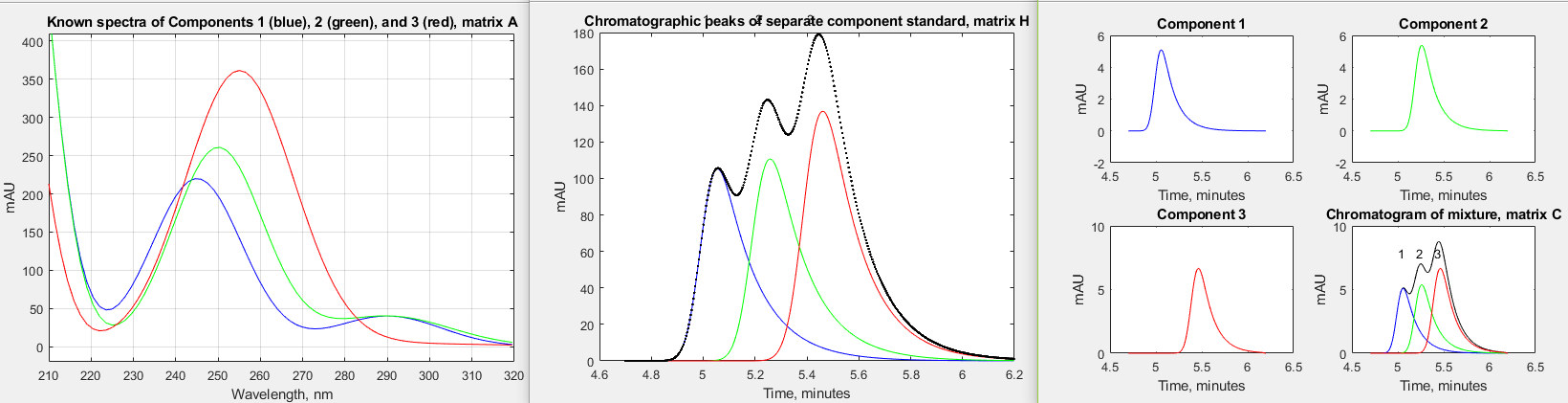
challenging variation on the first one; #2
has much more chromatographic peak overlap; #3 has much more
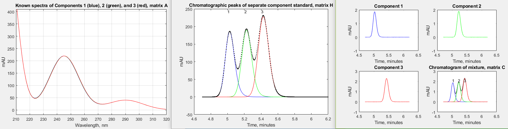
asymmetrical chromatographic peaks (higher tau); #4 has much more
similar spectra - in fact, the peak wavelengths differ by only
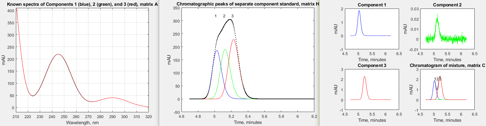
0.1 nm, making them look identical; in #5, component 2 (the
middle peak) has a concentration 100 times lower; and #6
is the same as #5 except that the peaks are highly asymmetrical.
In all of these cases, the normal perpendicular drop area
measurement technique is either impossible (because there are no
distinct peaks for each component) or are very much in error,
but the CLS techniques works well, giving very low errors except
when the middle peak concentration is 0.0001, which approaches
the random noise limit of the detector. (Another variation, TimeResolvedCLSbaseline.m,
includes the correction for baseline shifts.)
| Peak resolution |
Spectral similarity |
Peak asymmetry |
Concentration ratios |
% errors in area measurement |
Links |
| 1.
Normal |
Normal |
Slight:
tau=10 |
.05
.05 .05 |
0.0022%
0.002% 0.0016% |
Graphic
m file |
| 2.
Unresolved |
Normal | Slight: tau=10 | .01
.01 .01 |
-0.06% -0.053%
-0.041% |
Graphic
m file |
| 3.
Partly resolved |
Normal | Great:
tau=40 |
.05
.05 .05 |
-0.0004%
-0.013% -0.066% |
Graphic m file |
| 4. Unresolved | Almost
complete |
Slight: tau=10 | .01
.01 .01 |
0.054%
0.049%
0.04% |
Graphic m file |
| 5. Unresolved | Almost complete | Slight:
tau=10 |
.01
.0001 .01 |
0.026%
2.4%
0.019% |
Graphic m file |
| 6. Unresolved | Almost complete | Great: tau=40 | .01 .0001 .01 | -0.04%
-3.8%
-0.03% |
Graphic m file |
Even when the peaks are resolved well enough for the perpendicular drop method to work, it can suffer from interaction between adjacent peak heights; that is, a change in the peak height of one peak can affect the measurement of the area of adjacent overlapped peaks, because of shifts in the valley point between them. This is illustrated by TimeResolvedCLScalibration.m, which simulates the measurement of 10 different three-component mixtures similar to the above (but modified so perpendicular drop measurement is possible), where the concentrations vary independently and randomly over a 1 x 10⁻⁴ to 9.5 x 10⁻⁴ microgram/mL range, and then plots measured peak area vs concentration for each component. (Each time you run this, you will get a different mix of concentrations). Linear least-squares fits of peak area vs concentration are calculated, as shown below. In this typical example, the average absolute percentage error in area measurement for the perpendicular drop method is about 5%, with an R2 of 0.995, and for the CLS measurement is less than 1%, with an R2 of 0.9995. (Even if the detector noise (line 22) is set to zero in this simulation, the errors in the perpendicular drop method remain, because they are caused by overlap between adjacent peaks, rather than by noise).

Though clearly the CLS method is very effective, all of this really only
proves that the mathematics works well; the method
still has the serious limitation that it requires that the
spectra of all the components be known accurately. This
requirement can be met in some applications, but in liquid
chromatography there is a potential pitfall. If gradient
elution and/or temperature programming are used, and if
the spectra of those chemical compounds are sensitive to the
solvent and/or to temperature, for example shifting their
peaks slightly, then there will likely be additional errors in
the CLS procedure. Obviously this depends on the particular
chemical system and will have to be evaluated on a
case-by-case basis.