

Video Demonstration
The "enhance" command-line function
function
Enhancedsignal=enhance(signal,factor1,factor2,SmoothWidth)
Basic function for resolution enhancement by the even-derivative
method. The arguments factor1 and factor2 are the
weighting factors for the 2nd and 4th
derivatives. SmoothWidth is the width of the smoothing
function applied to the derivatives. Optimum values for factor1
and factor2 depend on the width and the shape of the peaks
in the signal, and also on the desired trade-off between
resolution enhancement (peak width reduction) and baseline
artifacts that are a by-product of the method. As a starting
point, a reasonable value for factor1 is PeakWidth2/25
and for factor 2 is PeakWidth4/833 for peaks of
Gaussian shape (or PeakWidth2/6 and PeakWidth4/700
for
Lorentzian peaks), where PeakWidth is the full-width at half
maximum of the peaks expressed in number of data points. The
easiest way to determine the optimum values for your data is to
use iSignal or InteractiveResEnhance, described below.
Interactive Resolution Enhancement using the iSignal
function
iSignal is a Matlab function
that performs resolution enhancement for time-series signals,
using the above enhance function, with keystrokes that allow you
to adjust the 2nd and
4th derivative
weighting factors and the smoothing continuously while observing
the effect on your signal dynamically. View the code here or dowload the ZIP file with sample data
for testing. Just place isignal.m in
the Matlab path and type
             >> isignal(DataMatrix); or
             >> isignal(x,y);  or
             >> isignal(y);
where DataMatrix is a matrix with x
values in the first row or column and y values in the
second. Press K
to see all the keyboard commands. Use the cursor arrow
keys to pan and zoom.
The E key turns
the resolution enhancement function on and off. iSignal is particularly
convenient to use because it calculates the sharpening and
smoothing settings for Gaussian and for Lorentzian peak
shapes using the Y and U keys,
respectively. Just isolate a single typical peak in the
upper window using the pan and zoom keys, then press Y for Gaussian or U for Lorentzian
peaks. (The optimum settings depends
on the width of the peak, so if your signal has peaks of
widely different widths, one setting will not be optimum for
all the peaks). You can fine-tune the sharpening with the F/V and G/B keys and the
smoothing with the A/Z keys. Press K to see all the keyboard
commands.
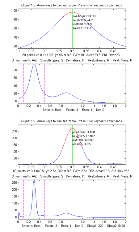
The graphic example on
the right is the result of the following commands:
>> x=[0:.005:2];y=humps(x);Data=[x;y];
>>
isignal(Data,0.3,0.5,1,3,1,0,1,220,5400);
Press the 'E' key to toggle sharpening ON/OFF to compare before
and after peak sharpening.
| Interactive optimization of derivative resolution enhancement for your own data. Requires Matlab 6.5. To use this, place the data to be enhanced in the global vector "signal", then execute this file. It plots the data and displays sliders for separate real-time control of 2nd and 4th derivative weighting factors (factor and factor2) and smooth width. (Larger values of factor1 and factor2 will reduce the peak widths but will cause artifacts in the baseline near the peak. Adjust the factors for the best trade-off). Use the minimum smooth width needed to reduce excess noise. The resolution-enhanced signal is placed in the global vector "Enhancedsignal". (If the range of the sliders is inappropriate for your signal, you can adjust the slider ranges in lines 27-29). |
| Self-contained demo of resolution enhancement for a simulated signal of four overlapping peaks. Requires Matlab 6.5. Displays sliders for separate real-time control of 2nd and 4th derivative weighting factors (factor and factor2) and smooth width. Larger values of factor1 and factor2 will reduce the peak width but will also cause artifacts in the baseline near the peak. Adjust these factors for the the best compromise. Use the minimum smooth width needed to reduce excess noise (too much smoothing will reduce the resolution enhancement). |
| Similar to DemoResEnhance, but for a single Gaussian peak. This allows you to experiment with the adjustable parameters that work best for a peak of Gaussian shape. You can change the width of the peak in line 26. The estimated width of the resolution-enhanced peak is computed and displayed above the graph, to make it easier to determine the extent of resolution enhancement quantitatively. Try to adjust the parameters until the estimated peak width is as small as possible, while still giving acceptable baseline flatness. |
| Similar to DemoResEnhance, but for a single Lorentzian peak. Requires Matlab 6.5. This allows you to experiment with the adjustable parameters that work best for a peak of Lorentzian shape. You can change the width of the peak in line 26. The estimated width of the resolution-enhanced peak is computed and displayed above the graph, to make it easier to determine the extent of resolution enhancement quantitatively. Try to adjust the parameters until the estimated peak width is as small as possible, while still giving acceptable baseline flatness. |


Number of unique visits since May 17, 2008: