Computations
carried
out by computer software with non-integer numbers have a
natural limit to the precision with which they can be
represented; for example, the number 1/3 is represented as
0.3333333... with a large but finite number of "3"s, whereas
theoretically there are an infinite string of "3"s
in the decimal representation of 1/3. It's the same with
irrational numbers such as "pi" and the square root of 2;
they can never have a exact decimal representation. In
principle, these tiny errors could accumulate in a very
complex multiple-step calculation and could conceivably become
a significant source of error. In the vast majority of
applications to scientific computation, however, these
limits will be minuscule compared to the errors and random
noise that is already present in most real-world
measurements. But it is best to know what those numerical
limits are, under what circumstances they might occur, and
how to minimize them.
Multicomponent
spectroscopy. Probably the most common calculation
where numerical precision is an issue is in the matrix
methods that are used in multicomponent
spectroscopy. In the derivation of the Classical
Least Squares (CLS) method, the matrix
inverse is used to solve large systems of
linear equations. The matrix inverse is a standard function
in programming languages such as Matlab, Octave,
Wolfram's Mathematica,
and in spreadsheets. But if you use that function in Matlab,
the function name ("inv") is automatically
flagged
by the editor with the following warning:
"For solving a system of linear equations, the inverse of a matrix is primarily of theoretical value. Never use the inverse of a matrix to solve a linear system Ax=b with x=inv(A)*b, because it is slow and inaccurate.... Instead of multiplying by the inverse, use matrix right division (/) or matrix left division (\). That is: Replace inv(A)*b with A\b...[and]...replace b*inv(A) with b/A"
 "Slow
and inaccurate"? OK, now I'm scared.
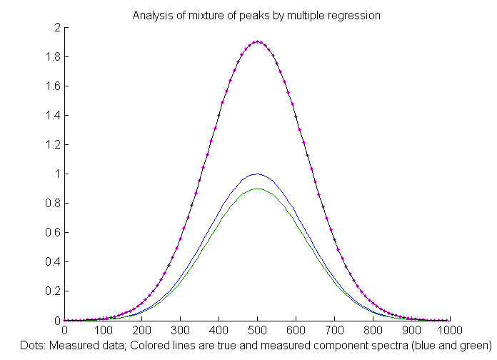
But how serious a problem is this really in actual
applications? To answer that question, the Matlab/Octave
script RegressionNumericalPrecisionTest.m
applies the CLS method to a mixture of two very
closely-spaced noiseless overlapping
Gaussian peaks (blue and green lines in the figure on the
left) using three different mathematical formulations of the
least-squares calculation that give different results. (The
peaks must not have any added random noise, because here we
are focusing on the errors caused by the computer itself
and not, as in everywhere else in this essay, on external
physical noise). The difficulty of such a measurement
depends on the ratio of the peak separation to the peak
half-width; small ratios mean very highly overlapped peaks
which are hard to measure accurately. In this example the
separation-to-width ratio is 0.0033, which is very small
(i.e. difficult); this is equivalent to trying to measure a
mixture of two absorption spectroscopy peaks that are 300 nm wide and separated
by only 1 nm, a
tiny difference that you
wouldn't even notice with the naked eye. The
results of this script shows that the matrix inverse ("inv")
method does indeed have an error
thousands of times larger than the method using matrix
division, but even the matrix division
error is still very small. Practically, the
difference between these methods is unlikely to be
significant when applied to real experimental data, because
even the tiniest bit of signal instability (like that caused
by small changes in the temperature of the sample or random
noise in the signal, which
you can simulate in line 15) produces a far greater error.
So basically that warning message is the voice of a
mathematician or computer programmer, not an experimental
scientist.
"Slow
and inaccurate"? OK, now I'm scared.
But how serious a problem is this really in actual
applications? To answer that question, the Matlab/Octave
script RegressionNumericalPrecisionTest.m
applies the CLS method to a mixture of two very
closely-spaced noiseless overlapping
Gaussian peaks (blue and green lines in the figure on the
left) using three different mathematical formulations of the
least-squares calculation that give different results. (The
peaks must not have any added random noise, because here we
are focusing on the errors caused by the computer itself
and not, as in everywhere else in this essay, on external
physical noise). The difficulty of such a measurement
depends on the ratio of the peak separation to the peak
half-width; small ratios mean very highly overlapped peaks
which are hard to measure accurately. In this example the
separation-to-width ratio is 0.0033, which is very small
(i.e. difficult); this is equivalent to trying to measure a
mixture of two absorption spectroscopy peaks that are 300 nm wide and separated
by only 1 nm, a
tiny difference that you
wouldn't even notice with the naked eye. The
results of this script shows that the matrix inverse ("inv")
method does indeed have an error
thousands of times larger than the method using matrix
division, but even the matrix division
error is still very small. Practically, the
difference between these methods is unlikely to be
significant when applied to real experimental data, because
even the tiniest bit of signal instability (like that caused
by small changes in the temperature of the sample or random
noise in the signal, which
you can simulate in line 15) produces a far greater error.
So basically that warning message is the voice of a
mathematician or computer programmer, not an experimental
scientist.
Analog-to-digital
resolution. 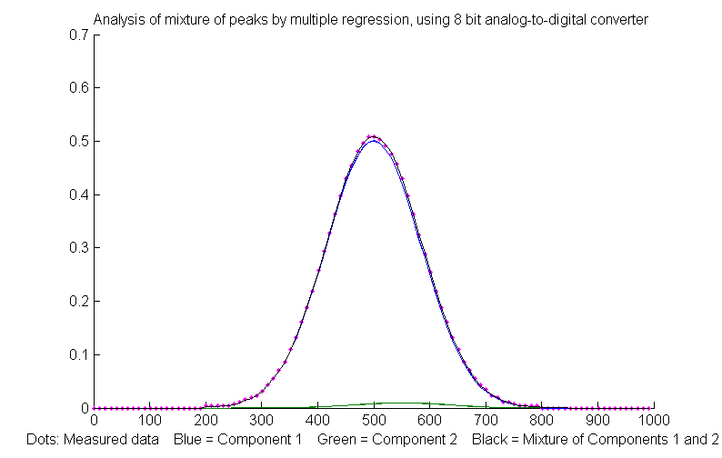 Potentially more
significant than the computer's numerical resolution is the
resolution of the analog-to-digital
converter (ADC)
that is used to convert analog signals (e.g. voltage) to a
number. The Matlab/Octave script RegressionADCbitsTest.m
demonstrates this, with two slightly overlapping Gaussian
bands with a large (50-fold)
difference
in peak height (blue
and
green lines in the figure on the right); in this case the
separation to width ratio is 0.25, much larger (i.e. easier)
than the previous example. For this example, the simulation
shows that the relative percent errors of peak height
measurement is 0.19% for the larger peak and 6.6% for the
smaller peak. You can change the resolution of the simulated
analog-to-digital converter in number
of
bits (line 9). The amplitude
resolution of an analog-to-digital converter is 2 raised to
the power of the number of bits. Common
ADC resolutions are 10, 12, and 14 bits, corresponding to
resolutions of one part in 1024, 4096 and 16384,
respectively. Of course, the effective resolution for the smaller
peak in this case is 50
times less, and you can't simply turn up the amplification
on the smaller peak without overloading the ADC for the
larger one.
Potentially more
significant than the computer's numerical resolution is the
resolution of the analog-to-digital
converter (ADC)
that is used to convert analog signals (e.g. voltage) to a
number. The Matlab/Octave script RegressionADCbitsTest.m
demonstrates this, with two slightly overlapping Gaussian
bands with a large (50-fold)
difference
in peak height (blue
and
green lines in the figure on the right); in this case the
separation to width ratio is 0.25, much larger (i.e. easier)
than the previous example. For this example, the simulation
shows that the relative percent errors of peak height
measurement is 0.19% for the larger peak and 6.6% for the
smaller peak. You can change the resolution of the simulated
analog-to-digital converter in number
of
bits (line 9). The amplitude
resolution of an analog-to-digital converter is 2 raised to
the power of the number of bits. Common
ADC resolutions are 10, 12, and 14 bits, corresponding to
resolutions of one part in 1024, 4096 and 16384,
respectively. Of course, the effective resolution for the smaller
peak in this case is 50
times less, and you can't simply turn up the amplification
on the smaller peak without overloading the ADC for the
larger one.
Surprisingly, if most of the noise in the signal is
this kind of digitization noise, it may actually help to add
some additional random noise (specified in line 10 in this
script), as was seen in appendix I.

Differentiation. 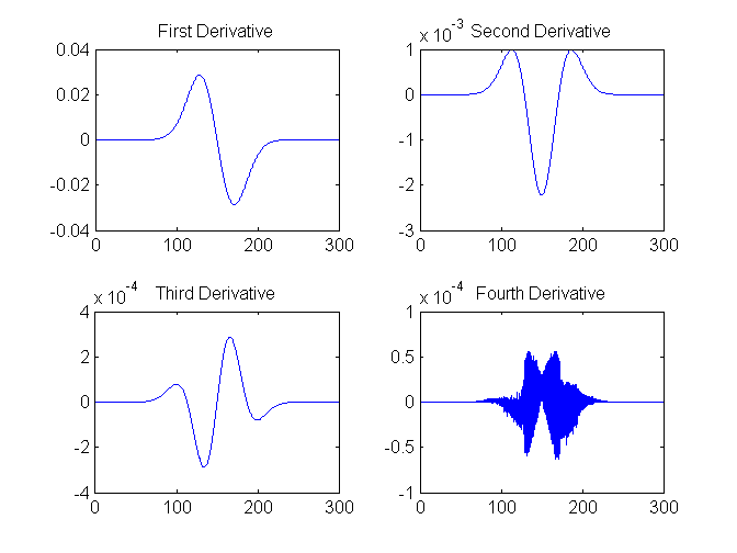 Another
application where you can see numerical precision noise is
in differentiation,
which involves the subtraction of very nearly equal adjacent
numbers in a data series. The self-contained Matlab/Octave
function DerivativeNumericalPrecisionDemo.m
shows how the numerical precision limits of the computer
effects the first through fourth derivatives of a Gaussian
band that is very finely
sampled (over 16,000 points in the half-width in this
case) and that has no added
noise. The plot on the left shows the four waveforms in
Figure 1, left, and their frequency spectra in Figure 2,
below. The numerical precision limits of the computer
creates random noise at very high frequencies, which are
emphasized by differentiation. In the frequency spectra
below, the big
low-frequency bump near a frequency of 10-2 is the signal and everything above
that is numerical noise. The
lower-order derivatives are seldom a problem, but by the
time you reach the fourth derivative, those noise
frequencies approach the strength of the signal frequencies,
as you can see in the frequency spectrum of the fourth
derivative in the lower right. But
this noise is only a very high-frequency noise, so smoothing
with as little as a 3-point sliding average smooth removes
most of it (click
to view).
Another
application where you can see numerical precision noise is
in differentiation,
which involves the subtraction of very nearly equal adjacent
numbers in a data series. The self-contained Matlab/Octave
function DerivativeNumericalPrecisionDemo.m
shows how the numerical precision limits of the computer
effects the first through fourth derivatives of a Gaussian
band that is very finely
sampled (over 16,000 points in the half-width in this
case) and that has no added
noise. The plot on the left shows the four waveforms in
Figure 1, left, and their frequency spectra in Figure 2,
below. The numerical precision limits of the computer
creates random noise at very high frequencies, which are
emphasized by differentiation. In the frequency spectra
below, the big
low-frequency bump near a frequency of 10-2 is the signal and everything above
that is numerical noise. The
lower-order derivatives are seldom a problem, but by the
time you reach the fourth derivative, those noise
frequencies approach the strength of the signal frequencies,
as you can see in the frequency spectrum of the fourth
derivative in the lower right. But
this noise is only a very high-frequency noise, so smoothing
with as little as a 3-point sliding average smooth removes
most of it (click
to view).

