


Appendix
M: Curve fitting in spreadsheets and stand-alone
programs.
Both Excel and OpenOffice
Calc have a "Solver"
capability that will change specified cells in an attempt to
produce a specified goal; this can be used in
peak fitting to minimize the fitting error between a set of
data and a proposed calculated model, such as a set of
overlapping Gaussian bands. (This external source, https://www.wallstreetmojo.com/solver-in-excel/,
has a detailed graphical explanation of using the
Solver.) Solver
includes three
different solving methods. This
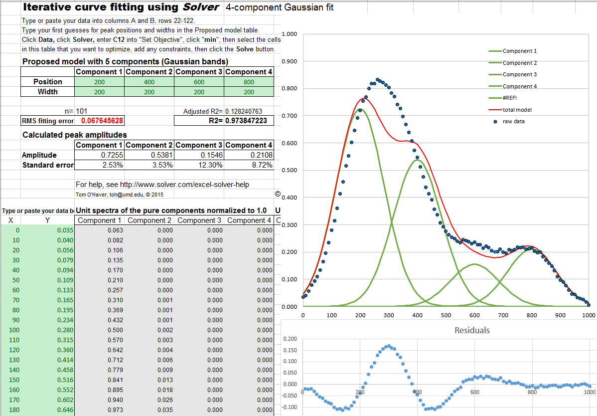
Excel spreadsheet example (screen shot) demonstrates how this is used to fit four Gaussian components to a
sample set of x,y data that has already been entered into columns
A and B, rows 22 to 101 (you could type
or paste in your own data there).

So, how many Gaussian components does it
take to fit the data? One way to tell is to look at the plot of
the residuals (which shows the point-by-point difference
between the data and the fitted model), and add components until
the residuals are random, not wavy, but
this works only if the data are not
smoothed before fitting. Here's an
example - a set of real data that are fit with an increasing
sequence of two
Gaussians, three Gaussians, four
Gaussians, and five Gaussians. As you look at this sequence of
screenshots, you'll see the percent fitting error decrease, the R2 value become closer
to 1.000, and the residuals become smaller and more random. (Note
that in the 5-component fit, the first and last components are not peaks within the 250-600 x range of the data,
but rather account for the background). There is no need to try a 6-component
fit because the residuals
are already random at 5 components and more components than that
would just "fit the noise" and would likely be unstable and give a
very different result with another sample of that signal with
different noise.
There
are a number of downloadable non-linear iterative curve fitting
adds-ons and macros for Excel and OpenOffice. For
example, Dr. Roger Nix of
Queen Mary University of London has developed a very nice Excel/VBA
spreadsheet for curve fitting X-ray
photoelectron spectroscopy (XPS) data, but it
could be used to fit other types of spectroscopic data. A 4-page
instruction sheet is also provided.
The Python language has many options for iterative
least-squares; one is is compared
to its Matlab equivalent.
There are also many
examples of stand-alone freeware and
commercial programs, including PeakFit, Data Master 2003, MyCurveFit, Curve Expert, Origin, ndcurvemaster,
and the R language.
If you use a spreadsheet for this type of curve
fitting, you have to build a custom spreadsheet for each
problem, with the right number of rows for the data and with the
desired number of components. For example, my CurveFitter.xlsx
template is only for a 100-point signal and a 5-component
Gaussian model. It's easy to extend to a larger number of data
points by inserting rows between 22 and 100, columns A through
N, drag-copying the
formulas down into the new cells (e.g. CurveFitter2.xlsx is
extended to 256 points). To handle other numbers of components
or model shapes you would have to
insert or delete columns between C and G and between Q and U
and edit the formulas, as has been done in this set of
templates for 2
Gaussians, 3 Gaussians, 4
Gaussians, 5 Gaussians,
and 6
Gaussians.
If your peaks are superimposed on a
baseline, you can include a model for the
baseline as one of the components. For
instance, if you wish to fit 2 Gaussian peaks on a linear
tilted slope baseline, select a 3-component spreadsheet
template and change one of the Gaussian components to the
equation for a straight line (y=mx+b, where m is
the slope and b is
the intercept). A template for that particular case is CurveFitter2GaussianBaseline.xlsx (graphic);
don't click "Make Unconstrained Variables Non-Negative" in
this case, because the baseline model may well need negative
variables, as it does in this particular example. If you want
to use another peak shape or another baseline shape, you'd
have to modify the equation in row
22 of the corresponding columns C
through G and drag-copy the modified cell down to the last
row, as was done to change the Gaussian peak shape into
a Lorentzian shape in CurveFitter6Lorentzian.xlsx.
Or you could make columns
C through G contain equations for different peak or baseline
shapes. For
exponentially broadened Gaussian peak shapes, you can use CurveFitter2ExpGaussianTemplate.xlsx
or two overlapping peaks (screen graphic). In this
case, each peak has four parameters: height, position, width,
and lambda (which determines the asymmetry - the extent of
exponential broadening).
In some cases, it is useful to add constraints
to the variables determined by iteration, for example to
constrain them to be greater than zero, or constrained between
two limits, or equal to each other, etc. Doing so will force
the solutions to adhere to known expectations and avoid
nonphysical solutions. This is especially important for
complex shapes such as the exponentially broadened Gaussian
just discussed in the previous paragraph. You can
do this by adding those constraints using the "Subject to the
Constraints:" box in the center of the "Solver Parameters" box
(see the graphic above). For details, see https://www.solver.com/excel-solver-add-change-or-delete-constraint?
The point is that you can do - in fact, you must do - a lot of
custom editing to get a spreadsheet template that fits your
data. In contrast, my Matlab/Octave peakfit.m function
automatically adapts to any number of data points and is
easily set to over 40 different model peak shapes and any
number of peaks simply by changing the input arguments. Using
my Interactive Peak Fitter function ipf.m in Matlab, you can press a single
keystroke to instantly change the peak shape, number of peaks,
baseline mode, or to re-calculate the fit with different start
or with a bootstrap subset of the data. That's far quicker and
easier than the spreadsheet. But on the other hand, a real advantage of spreadsheets in this
application is that it is relatively easy to add your own custom shape functions
and constraints, even complicated ones, using standard
spreadsheet cell formula construction. And if you are hiring
help, it's probably easier to find an experienced spreadsheet
programmer than a Matlab programmer. So, if you are not sure
which to use, my advice is to try both methods and decide for
yourself.
This page is part of "A Pragmatic Introduction to Signal
Processing", created and maintained by Prof. Tom O'Haver ,
Department of Chemistry and Biochemistry, The University of Maryland
at College Park. Comments, suggestions and questions should be
directed to Prof. O'Haver at toh@umd.edu. Updated July, 2022.