The random walk was mentioned
in the section on signals and noise as a type of
low-frequency ("pink") noise. Wikipedia says:
"A
random walk is a mathematical formalization of a path that
consists of a succession of random steps. For example, the path
traced by a molecule as it travels in a liquid or a gas, the
search path of a foraging animal, "superstring" behavior, the
price of a fluctuating stock and the financial status of a
gambler can all be modeled as random walks, although they may
not be truly random in reality."
Random walks describe and serve as a model for many kinds
of unstable behavior. Whereas white, 1/f, and blue noises are
anchored to a mean value to which they tend to return, random
walks tend to be more aimless and often drift off on one or
another direction, possibly never to return. 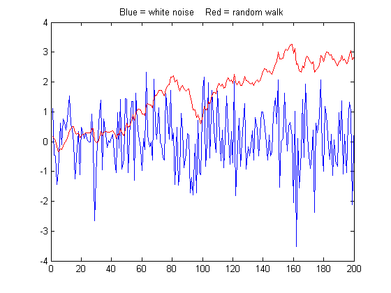 Mathematically, a
random walk can be modeled as the cumulative sum of some random
process, for example the 'randn' function. The graph on the
right compares a 200-point sample of white noise (computed as
'randn' and shown in blue) to a random
walk (computed as a cumulative sum, 'cumsum', and shown in red). Both samples are scaled to
have exactly the same standard deviation, but even so their behavior is vastly different. The
random walk has much more low frequency behavior, in this case
wandering off beyond the amplitude range of the white noise.
This type of random behavior is very disruptive to the
measurement process, distorting the shapes of peaks and causing
baselines to shift and making them hard to define, and it can
not be reduced significantly by smoothing (See NoiseColorTest.m).
In this particular example, the random walk has an overall
positive slope and a "bump" near the middle that could be
confused for a real signal peak (it's not; it's just noise). But
another sample might have very different
behavior. Unfortunately, it is not
uncommon to observe this behavior in experimental signals.
Mathematically, a
random walk can be modeled as the cumulative sum of some random
process, for example the 'randn' function. The graph on the
right compares a 200-point sample of white noise (computed as
'randn' and shown in blue) to a random
walk (computed as a cumulative sum, 'cumsum', and shown in red). Both samples are scaled to
have exactly the same standard deviation, but even so their behavior is vastly different. The
random walk has much more low frequency behavior, in this case
wandering off beyond the amplitude range of the white noise.
This type of random behavior is very disruptive to the
measurement process, distorting the shapes of peaks and causing
baselines to shift and making them hard to define, and it can
not be reduced significantly by smoothing (See NoiseColorTest.m).
In this particular example, the random walk has an overall
positive slope and a "bump" near the middle that could be
confused for a real signal peak (it's not; it's just noise). But
another sample might have very different
behavior. Unfortunately, it is not
uncommon to observe this behavior in experimental signals.
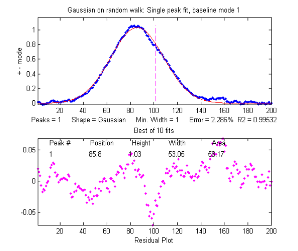
To demonstrate the measurement difficulties, the script RandomWalkBaseline.m
simulates a Gaussian peak with randomly variable position and
width, on a random walk baseline, with a S/N ratio is 15. The
peak is measured by least-squares curve fitting methods using peakfit.m with two
different methods of baseline correction in an attempt to handle
the random walk:
(a) a single-component Gaussian model (shape 1) with autozero set to 1 (meaning a linear baseline is first interpolated from the edges of the data segment and subtracted from the signal): peakfit([x;y],0,0,1,1,0,10,1);
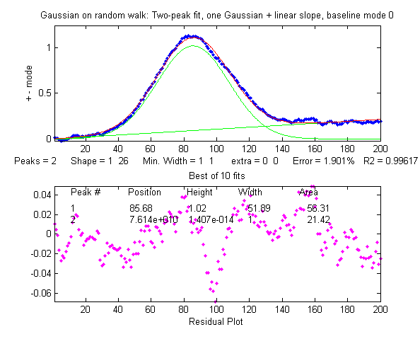
(b) a 2-component model, the first being a Gaussian (shape 1) and the second a linear slope (shape 26), with autozero set to 1: peakfit([x;y],0,0,2,[1 26],[0 0],10,0).
In this particular case the fitting error is lower for the second method, especially if the peak falls near the edges of the data range.
But the
relative percent errors of the peak parameters show that the first method gives a
lower error for position and width, at least in this case. On
average, the peak parameters are about the same.
Position Error
Height Error Width Error
Method a: 0.2772
3.0306 0.0125
Method b: 0.4938
2.3085 1.5418
You can compare this to WhiteNoiseBaseline.m
which has a similar signal and S/N ratio, except that the noise
is white.
Interestingly, the fitting error
with white noise is greater, but the parameter errors (peak position,
height, width, and area) are lower, and the residuals are more random and less likely to
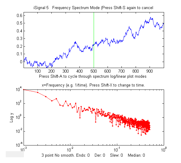
produce false noise peaks. This is because the random walk noise
is very highly concentrated at low frequencies where
the signal frequencies usually lie, whereas white noise also has
considerable power at higher
frequencies, which increases the fitting error but does comparatively little damage to signal
measurement accuracy. This may be slightly counter-intuitive,
but it's important to realize that fitting error does not always
correlate with peak parameter error. Bottom line: random
walk is troublesome.
Depending on the type of experiment, an instrumental design
based on modulation techniques may help, and
ensemble averaging multiple
measurements can help with any type of unpredictable random
noise, which is discussed in the very next section.
This page is part of "A Pragmatic Introduction to Signal
Processing", created and maintained by Prof. Tom O'Haver ,
Department of Chemistry and Biochemistry, The University of
Maryland at College Park. Comments, suggestions and questions
should be directed to Prof. O'Haver at toh@umd.edu. Updated July, 2022.