This appendix examines
more closely the question of measuring peak area
rather than peak height to reduce the effect of peak
broadening, which commonly occurs in chromatography,
for reasons that are discussed previously,
and also in some forms of spectroscopy. Under what
conditions the measurement of peak area might be
better than peak height?
The Matlab/Octave script "HeightVsArea.m" simulates the measurement of a series of
standard samples whose concentrations are given by the
vector 'standards'. Each standard produces an isolated
peak whose peak height is directly proportional to the
corresponding value in 'standards' and whose underlying shape is a Gaussian with a constant peak
position ('pos') and width ('wid'). To simulate the
measurement of these samples under typical conditions,
the script changes the shape of the peaks (by
exponential broadening) and adds a variable baseline
and random noise. You can control, by means of the
variable definitions in the first few lines of the
script, the peak beginning and end, the sampling rate
'deltaX' (increment between x values), the peak
position and width ('pos' and 'wid'), the sequence of
peak heights ('standards'), the baseline amplitude
('baseline') and its degree of variability ('vba'),
the extent of shape change ('vbr'), and the amount of
random noise added to the final signal ('noise').
The resulting peaks a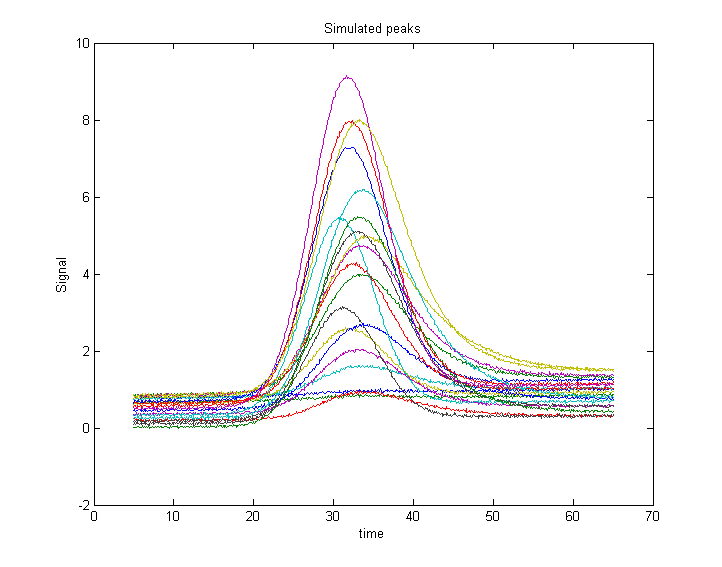 re shown in Figure 1. The script prepares a
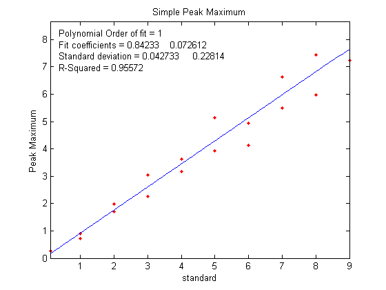
series of "calibration curves"
plotting the values of 'standard' against the measured
peak heights or areas for each measurement method. The
measurement methods include peak height in Figure 2,
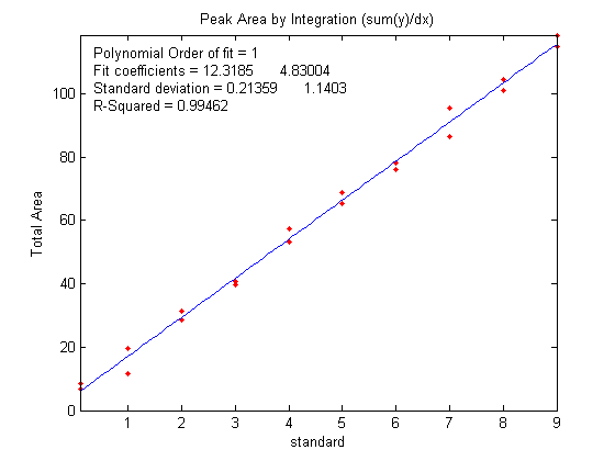
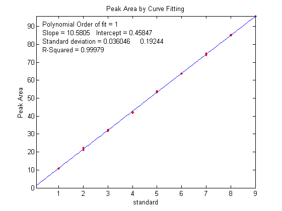
peak area in Figure 3, and curve
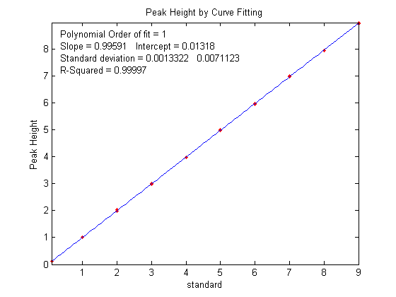
fitting height and area in Figures
4 and 5, respectively. These
plots should ideally have an intercept of zero and an R2 of 1.000, but the slope is greater for the peak area measurements
because area has different units and is numerically
greater than peak height. All the measurement methods
are baseline corrected; that is, they include code
that attempts to compensate for changes in the
baseline (controlled by the variable 'baseline').
re shown in Figure 1. The script prepares a
series of "calibration curves"
plotting the values of 'standard' against the measured
peak heights or areas for each measurement method. The
measurement methods include peak height in Figure 2,
peak area in Figure 3, and curve
fitting height and area in Figures
4 and 5, respectively. These
plots should ideally have an intercept of zero and an R2 of 1.000, but the slope is greater for the peak area measurements
because area has different units and is numerically
greater than peak height. All the measurement methods
are baseline corrected; that is, they include code
that attempts to compensate for changes in the
baseline (controlled by the variable 'baseline').
With the initial values of 'baseline',
'noise', 'vba', and 'vbr', you can clearly see the
advantage of peak area measurements (figure 3)
compared to peak height (figure 2). This is primarily
due to the effect of the variability of peak shape
broadening ('vbr') and to the averaging out of random
noise in the computation of area.
If you set 'baseline', 'noise', 'vba', and 'vbr' all to zero, you've simulated a perfect world in which all methods work perfectly.
Curve fitting
can measure both peak height and area; it is not even absolutely
necessary to use an accurate peak shape model. Using a simple Gaussian model in this example
works much better for peak area (Figure 5) than for peak height (Figure
4) but is not significantly better than a simple
peak area measurement (Figure 3). The best results are
obtained if an exponentially-broadened Gaussian model (shape 31 or 39) is used,
using the code in line 30, but that computation takes
longer. Moreover, if the measured peak overlaps another peak significantly, curve fitting both
of those peaks together can give much more accurate results that other peak area measurement methods.
This page
is part of "A Pragmatic Introduction to Signal
Processing", created and maintained by Prof. Tom O'Haver ,
Department of Chemistry and Biochemistry, The University of
Maryland at College Park. Comments, suggestions and questions
should be directed to Prof. O'Haver at toh@umd.edu. Updated July, 2022.