This is a simulation of the spectroscopy of a line-source atomic
absorption (AA) measurement. It is not a simulation of an AA
instrument. What's the difference? An
instrument simulation shows you how to work an AA instrument.
This simulation shows you how AA spectroscopy works,
that is, what goes on under the instrument's surface. So much is
hidden from the observer in AA spectroscopy; with a typical
line-source instrument, it is not even possible to scan the
spectrum of the light source or the absorber with sufficient
resolution to see what is going on.
The purpose of the simulation is to make it clearer how the
various spectroscopic aspects relate to each other and to the
measured absorbance, in a line-source atomic absorption
measurement with continuum-source background correction in a
steady-state (i.e. flame) atomizer. You can observe the
spectral relationship of the hollow
cathode lamp emission profile to the atomic absorption
profile, observe the effect of different spectral line
widths of both the absorbing atom and the hollow cathode
lamp, correction of background absorption by continuum-source (D2)
method, over-correction caused by structured background
absorption, and the effect of non-absorbing lines, line-overlap
interferences, and hyperfine
structure.
Several simplifying assumptions are made, which do not impact the
main points to be made. In this simulation, the atomic absorption
lines are modeled as a Lorentzian (although the actual
line shape depends on the relative contributions of Doppler and
collisional (pressure) broadening, both of which temperature
and pressure dependent. The hollow cathode lamp's line is
modeled as a Gaussian (temperature-broadened only, not
pressure broadened, due to the low internal pressure of the lamp).
Background absorption is assumed to be constant over the spectral
bandwidth of the spectrometer, which is fixed at 0.2 nm. The
simulation is meant to be generic for any typical element, not
tailored to the specific spectroscopic properties of any one
element. Hence, the wavelength scale (x-axis) is relative to the
atomic line center and extends positive and negative from that.
INPUTS: shift = collisional shift of absorption line, pm. abs. width = spectral width of atomic absorption line, pm. source width = spectral width of hollow-cathode lamp emission line, pm. atom density = relative concentration of atoms in atomizer, arbitrary units. stray light = relative intensity of continuum background radiation from hollow-cathode lamp. background abs. = non-specific background absorption in atomizer. non-abs. line = intensity of a non-absorbing line from HCL. arbitrarily placed at -60 pm, relative to main resonance line. interference = peak absorbance of matrix absorption line, arbitrarily placed at +60 pm. hyperfine = relative intensity of hyperfine line, relative to main resonance line.
Array calculations:
A39..A139: wavelength = -100 to +100 (displacement in pm from resonance wavelength) Total number of wavelength intervals = NumWavelengths
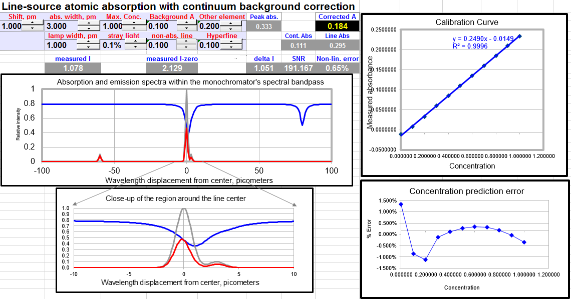
Graph shows spectral profile in region ±100 pm around resonance line.
Gray line: SourceIntensity Blue line: transmission Red line: TransmittedIntensity
OUTPUTS: Peak abs. = "true" peak absorbance at center of absorption line. Width ratio = ratio of absorption width to source width. Cont. A = absorbance measured with continuum source. Uncorr. A = absorbance measured with line source. Corrected A = atomic absorbance corrected for background absorbance (equals Uncorr. A - Cont. A). measured I = total intensity transmitted through atomizer, measured at the detector over the entire spectral bandpass. measured I-zero = total incident intensity measured at detector over entire spectral bandpass. delta I = difference between measured I-zero and measired I. SNR = signal-to-noise ratio for photon-limited measurement.
Display calculations:
measured I = MeasI = sum(TransmittedIntensity) measured I-zero = MeasIzero = sum(SourceIntensity) delta I = MeasIzero-MeasI SNR = 1000*CorrectedA*sqrt(MeasI) Peak abs. = Conc/(AbsWidth) Width ratio = SourceWidth/AbsWidth Cont. A = Ac =log((NumWavelengths))/(sum(transmission))) Line A = Al = log(MeasIzero/MeasI) CorrectedA = Al-Ac
Operating Instructions
Computer Simulation of
the Spectroscopy of Atomic Absorption
The graph displays a plot
of intensity on the y axis vs wavelength displacement from the
resonance wavelength, in pm, on the x axis. The x axis extends
over the spectral bandpass of the monochromator (0.2 nm, or 200
pm, in this case), which is centered on the resonance wavelength.
There are three lines on the plot in different colors: the
spectral profile of the incident line-source emission line (gray),
the analyte transmission profile (blue), and the spectral profile
of the transmitted line-source emission line (red). (In a real AA
instrument you actually wouldn't be able to see these spectral
profiles, so in that respect this simulation is more instructive
that a real instrument). The purpose of the simulation is to make
it clearer how the various spectroscopic aspects relate to each
other and to the measured absorbance. In particular, this
simulation assumes an instrument with a continuum- source
background correction in a steady-state (i.e. flame) atomizer. The
input parameters that you have direct control over are displayed
at the top of the screen in the boxed cells with red
labels:
shift
Collisional ("red") shift of the absorption line, pm.
abs. width
Spectral width of the the analyte's atomic absorption
line, pm.
source width
Spectral width of the hollow-cathode lamp emission line,
pm.
atom density
Relative atom density of analyte atoms, arbitrary units.
stray light
Relative intensity of continuum background radiation from
the
hollow-cathode lamp.
background
abs.
Absorbance of the non-specific background absorption in
the atomizer
non-abs. line
Intensity of a non-absorbing line from the HCL,
arbitrarily
placed at -60 pm, relative to the main resonance line.
interference
Peak absorbance of a matrix absorption line, arbitrarily
placed
at +60 pm, relative to the main resonance line.
hyperfine
Relative intensity of the hyperfine line, relative to
intensity
of the "main" line.
To change any of these
parameters, click on the number, type in a new value, and press
the ENTER key. Recalculation is automatic.
The calculated "outputs"
are shown in the black boxes with white numbers and blue labels:
Peak abs.
The "true" peak absorbance at the center of
the absorption line.
Width ratio
Ratio of the absorption width to the source width.
Cont. A
Absorbance measured with the continuum source.
Line A
Absorbance measured with the line source.
Corrected A
Atomic absorbance corrected for background absorbance.
(This is simply equal to Line A - Cont. A).
measured I
Total intensity transmitted through the atomizer measured
over the entire spectral bandpass.
measured I-zero
Total incident intensity measured over the
entire spectral bandpass.
delta I
Difference between measured I-zero and measured I.
SNR
Theoretical signal-to-noise ratio for photon-noise-limited
measurement.
Of course in a real AA
instrument you wouldn't get all these outputs: usually only the
uncorrected and corrected absorbances are displayed. On some
instruments you can read the background absorbance (Cont A) and
the intensities (measured I or measured I-zero). No instrument
displays the true peak absorbance (it's fundamentally unknown),
the width ratio, or the theoretical SNR.
There are also two buttons
that automatically acquire an analytical curve:
Run calib. curve
Varies the atom density from 0 to 10 units in steps of 1
and
records the corrected
absorbance.
Plot and fit
Plots the resulting analytical calibration curve on a
separate sheet, fits a straight line to the low absorbance
(linear) region, and displays the slope and intercept of the
line.
If the analytical curve is
linear over the range of expected sample concentrations, then you
can calibrate the instrument by running a single standard solution
to determine the proportionality constant between concentration
and absorbance, then use that factor to convert the absorbance
readings on unknown samples into concentration. If the
analytical curve is not linear over the range of expected sample
concentrations, then you must calibrate the instrument by running
a series of standard solutions over that range range and plotting
absorbance vs standard concentration. This curve is then
used to convert the absorbance readings on unknown samples into
concentration.
Note than this simulation does not have a slit width control.
Line-source atomic absorption is different than other forms of
absorption spectroscopy because the primary light source is an atomic line source (e.g.
hollow cathode lamp or electrodeless discharge lamp) whose
spectral width is not a function of the monochromator slit width,
but rather is controlled by the temperature and pressure within
the lamp and by the hyperfine splitting of that element. The
only control that the operator has over the source line width is
the operating current of the lamp; increased current causes
increased temperature and pressure, both of which lead to
increased line width (increased source width), as well a higher
lamp intensity. So, to that extent, the effect of increasing
the lamp current is a bit like the effect of increasing the slit
width in a continuum-source absorption instrument; the intensity
goes up (good) but the increased source width and increasing
polychromatic effect causes calibration non-linearity (bad).
The slit width on a line-source atomic absorption instrument is
also adjustable by the user, but it has no effect on the source
width, being much greater (by 1000-fold or so) than the actual
line width of the atomic line source. (Typical atomic line
width 0.001 - 0.003 nm, compared to typical spectral bandpass of 1
nm). Increasing the slit width does increase the light intensity
linearity (because the entrance slit area increases directly), but
operating a too large a slit width runs the risk of increasing the
stray light, by allowing in other lines emitted by the atomic line
source that are not absorbed by the analyte in the atomizer, such
as lines originating from the fill gas, impurities in the lamp,
and non-resonance lines of the analyte. As always, stray
light leads to non-linearity, especially at high concentrations
and eventually to a plateau in the calibration curve at high
absorbances.
Student Assignment
Open the file
"AAMeasurement.wkz".
1. Make sure that all the
input parameters are set to their default values: shift =1, abs.
width = 3.5, source width = 1, and atom density = 1, and all other
inputs = 0. (These source and absorption widths are typical values
for the Ca 422 nm resonance line).
2. Note that the line
source absorbance (Line A) is slightly lower that the Peak abs.
Why? Does this lead to inaccuracy in analytical applications?
3. Increase atom density
to 10. Note that Peak abs. increases by exactly 10 as it should.
Did the line source absorbance (Line A) also increase by ten-fold?
Why not?
4. Note that the Corrected
A is lower that Line A, because the continuum source absorbance
Cont. A is not zero. Why is this so? To check that it is not an
offset or zero-adjust problem, set atom density to zero and verify
that all absorbances are zero. Does this have an effect on the
analytical linearity also? To test that, compare the corrected and
uncorrected absorbances at atom density of 1 and 10.
5. Return the atom density
to 1. To demonstrate that background correction is necessary,
increase the background abs. and notice the effect on Cont. A,
Corrected A and Line A. (In this idealized simulated instrument,
misalignment between the hollow cathode and continuum lamps is not
included, so the correction is perfect; it is never this perfect
in practice). Note that although the correction is perfect, the
SNR degrades (decreases) when the background absorbance increases.
Why?
6. Return the background
abs. to 0 and increase the interference, which controls the peak
absorbance of a matrix absorption line that falls within the
spectral bandpass but does not overlap the analytical absorption
line. Note that the Line A is not much changed, but the Cont. A,
and thus the Corrected A, is. Why? If only this kind of
interference occurs in a particular application, would it be more
accurate to use the corrected or uncorrected (line) absorbance for
analytical purposes? How do the Zeeman and pulsed HCL methods
minimize this problem?
7. Return the interference
to 0. Set non-abs line to 0.1. This controls the relative
intensity of a nonresonance (non-absorbing) line emitted by the
hollow cathode lamp that falls within the spectral bandpass. Note
the effect on the absorbances. Click on the Run calib. curve
button and, when it is finished running through all the atom
densities, click on the Plot and fit button to see the resulting
analytical curve. Explain the shape of the analytical curve.
(Note: each analytical curve plot is placed in a separate window,
to allow two or more to be compared; to discard them, click in the
close box in the upper left, the click in NO on the following
dialog box).
8. Return the non-abs line
to 0. Set hyperfine to 0.5 and notice the effect of the
transmission profile and the source line profile. Do an experiment
to determine if the presence of hyperfine structure influences the
sensitivity or linearity. What happens if hyperfine = 1? 9. Return
hyperfine to 0. All parameters should now be back at their default
values. Determine by experiment the absorbance that gives the best
SNR. Do your results agree with Ingle and Crouch for a photon
(shot) noise limit? See page 284 of James D. Ingle, Jr. and
Stanley R. Crouch, Spectrochemical Analysis, Prentice Hall, New
Jersey, 1988. (c) 1991, 2015. This page is part of Interactive
Computer Models for Analytical Chemistry Instruction, created
and maintained by Prof.
Tom O'Haver, Professor Emeritus, The University of Maryland at
College Park.
Comments, suggestions and questions should be directed to Prof.
O'Haver at toh@umd.edu.