The Retirement Simulation Spreadsheet

Tom O'Haver, University of Maryland, February 1998.
Dutch translation by Johanne Teerink.
 

This simulation shows how much income you can withdraw from a retirement account of $1,000,000 (e.g. an IRA or 401k account) that is invested it in any combination of fixed-interest or variable (equity) instruments, assuming that all interest and capital gains are re-invested and not taxed. You can control the income withdrawn, the rate of inflation, the return on your investments, and the volatility (uncertainty) of the equiry portion of the investment. Graphs show the variation of principal and yearly income vs time for a 35-year period.

Why $1,000,000? Because that amount is a long-term investment goal of many working people today and because most retired couples can live quite confortably on the income generated by the returns from an investment of that size.

This simulation is available in three different spreadsheet formats:

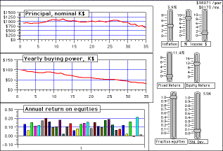
The WingZ version (screen shot shown) was developed using WingZ 1.1, an object-oriented spreadsheet with a powerful built-in macro language, that is available for Windows, Macintosh, and UNIX from Investment Intelligence Systems Corp. This is the only version that has mouse-controlled sliders for input control. You must own a copy of WingZ 1.1 to run this version. You may download the simulation in binary or HQX format.

The Excel version was developed in Microsoft Excel 3.0. You must own a copy of Microsoft Excel 3.0 or higher to run this version. You may download the Excel version of the simulation in binary or HQX format.

The Works version was developed in Microsoft Works 3.0. You must own a copy of Microsoft Works 3.0 or higher to run this version. You may download the Works version of the simulation in binary or HQX format.

The Input Variables:

• Inflation: This variable allows you to simulate the effects of inflation. Set it to the expected annual inflation rate. In the WingZ version, this variable is controlled by a slider with a range of 0 to 8% per year.
  
  
• Income: These two variables allow you to control the amount that you withdraw each year as income. The % income variable sets your annual income as a percentage of the total principal. The $ income variable sets your income as an inflation-adjusted dollar amount, independent of principal. You may use either one or any combination of these two variables to determine your income. The total income is the sum of the contributions of the two variables. The annual and monthly income for the first year is displayed in the top right corner.
  
  
• Fixed Return: The average annualized return on the fixed-interest portion of your investment portfolio (such as bonds or certificates of deposit), assuming that all interest and capital gains are re-invested and not taxed. In the WingZ version, this variable is controlled by a slider with a range of 0 to 8%.
  
  
• Equity Return: The average annualized return on the equity (stock and stock fund) portion of your investment portfolio, assuming that all interest and capital gains are re-invested and not taxed. Returns on equity investments are typically greater than that on fixed investments, but the returns fluctuate from year to year more than fixed investments. In the WingZ version, this variable is controlled by a slider with a range of 0 to 16%.
  
  
• Fraction in equities: The fraction of your portfolio's value that is invested in equities (stocks and stock funds). If you set this to zero, it means that all your portfolio is in fixed investments (an very conservative stance); if it is set to 1, all your investments are in equities (a higher-risk stance).
  
  
• Volatility. This simulates the volatility of the equity portion of your portfolio, by controlling the standard deviation of the equity returns. If you set this to zero, it means that there is no fluctuation in the returns (an unrealistic supposition). Volatility is measured in "standard deviation". In the WingZ version, this variable is controlled by a slider with a range of 0 - 60%.

• Principal, thousands $: The total value, in thousands of dollars, of your invested principal. The x-axis is the number of years of retirement. This starts out at $1,000,000.

• Annual income, K$: This is your total gross (pre-tax) inflation-adjusted yearly income, in thousands of dollars. It represents actual buying power of your income. The x-axis is the number of years of retirement. If your principal is held in a tax-deferred retirement account (e.g. an IRA or company-sponsored qualified 401k plan), you will have to pay ordinary income taxes on this income. If your principal is held in a Roth IRA account, you will have already paid the income taxes and therefore this represents your after-tax (take home) income.

• Annual return on equities: The simulates the year-to-year variation in the annualized return on the equity (stock and stock fund) portion of your investment portfolio. The average is controlled by the "Equity Return" variable and the fluctuation (variation) is controlled by the "Volatility" variable. Every time you recalculate the spreadsheet, another random set of returns is calculated.
  

1. Start with all the variables set to zero. Obviously in this case you are taking no income, so the income graph stays at zero and principal graph stays at $1,000,000.
   
   
2. Increase the $ income variable and notice the effect: the annual income graph is a flat line (constant) and the principal graph is a straight line sloping down, showing the depletion of principal. Set the $ income to $100,000/year. In this case you can do the math in your head - you are obviously going to run out of money in 10 years, and this is shown by the graphs as you would expect. Question: What is the largest annual income you can take that will cause your money to last for at least 35 years? Do you consider that a reasonable annual income for someone starting out with a million dollars?

3. Return the $ income to zero. Increase the % income and notice the effect: the both the annual income graph and the principal graph are now curved lines. This is because the income is calculated as a fixed percentage of the principal, so as the principal is depleted, income drops. If you set the $ income to $100,000/year, you will see that you don't run out of money suddenly; rather, your annual income decreases substantially with time as the principal is depleted.

4. So far, the inflation has been set to zero - that is, we have neglected the effects of inflation. Inflation has ben running about 2.5% per year in the last few years and has averaged about 3.5% over the last 15 years. Try setting the inflation between 3 and 4% and note the effect. It causes your income to decrease as inflation increases, because the income reported here is "inflation adjusted" - that is, expressed in the constant dollars of the first year of the simulation. The income graph is therefore an indication of the actual buying power of your income, which declines as inflation increases. No matter what the rate of inflation, one dollar of inflation adjusted income has the same buying power in the first year or in the 35^th year.

5. Now let us assume that you have invested your entire principal in a fixed-return account earning 5% yearly. Set the "Fixed Return" variable to 5. Set your annual income to $30,000. Now the principal graph shows an upward curve as the interest from your investment, compounded from year to year, more than compensates for the $30,000 annual income withdrawn. You could now increase your income without running out of money. Question: What income can you take that will cause your principal to remain unchanged for the full 35 year duration of the simulation? Limiting your income to this amount, you will never run out of money, no matter how long you live, and you will have all of the original principal to pass on to your heirs. However, perhaps you do not care to leave anything behind, in which case you can increase your income even further.

6. Typically, returns on equity investments (stocks and stock mutual funds) are greater than that for fixed investments. The long-term historical average annual return of the stock market is 10% including the Great Depression and 12% excluding the Depression. To simulate investment in equities, set the "Fraction in equities" variable to 1.0 and the "Equity Return" to between 10% to 12%. Question: Now what annual income can you take that will leave your principal unchanged?
   
   
7. The down side of investing in equities is the risk of fluctuating returns (called "volatility"). In some years the stock market does better than in other years. The volitility is the degree to which the returns fluctuate around their average; it is expressed in terms of standard deviation. The higher the standard deviation, the higher the fluctuation.

   What are the values of typical standard deviations? The standard deviation of the S&P 500 index varies between 10% and 16%, depending upon what time period is analyzed.^{1 - 3} Measured by the Vanguard 500 index fund, it was 10.2% over the past five years.⁴ Because of the "random walk" nature of stock market returns, the standard deviation typically increases with the time period analyzed; that is, standard deviations over a 10-year period are usually greater than those calculated over a shorter period. Between 1926 and 1994 the Dow Jones Industrial Average has had an average annual standard deviation of 20.30%. ⁵ Individual stocks can have even larger standard deviations.

   The problem with these fluctuation is that it makes long-term planning difficult. You can simulate the effect of these fluctuations by setting the "Volatility" variable to some non-zero value. Doing so will introduce some "bumpiness" in the principal curve (and in the income curve, if you are basing all or some of your income on a percentage of principal). Every time you you recalculate the spreadsheet, another random set of returns is calculated. This is like simulating various alternative possible "futures". Obviously this fluctuation makes precise planning impossible.

   But there is another and even more serious problem. If the standard deviation is suficiently large relative to the average return, it is possible that your principal may be exhausted within you life expectancy. Try increasing the volatility and see if you can observe such a "go broke" scenario. Obviously, you want to eliminate this possiblity. There are several ways to reduce the likelyhood of going broke: you could reduce your annual income, increase the rate of return on your investment returns, or reduce the volatility of your investment returns. Unfortunately, it is often true that the investments with the highest potential rate of return are the ones with the highest volatility; fixed return investments, which have the lowest volatility, typically have lower returns than equities.

8. The effect of volatility depends on whether you take your income as a percentage of principal or as a fixed dollar amount. To demonstrate this, try the following experiment. Set the standard deviation to zero and the % income to zero. Then adjust the $ income until the principal is just exhausted in year 35. Now increase the standard deviation to 5% and note the large effect. Now set the % income to this same income and set the $ income to zero. Recalculate the spreadsheet and note the greater stability of you income in the later years. In effect, this strategy reduces your income when investment returns are low and increases it when returns are high, greatly reducing the chance that you will go broke.

9. One way of reducing the risk of investing in stocks is to buy stock mutual funds^6-10. Individual stocks may have long- term standard deviations or 20% or more. Good quality mutual finds reduce risk by spreading your investment over many stocks and by seeking to increase returns by carefully selecting the stocks. What are the typical returns and variations in returns (volatility) of stock funds? The table below lists the performance of sixteen mututal funds and variable annuities over the last 10 years, listing the average annualized return and the standard deviation of the annual returns over that period. (Most published standard deviations are calculated from monthly results over a 3-year period and tend to be smaller than the numbers in this table. For example, the average standard deviation reported by Morningstar for the 171 small-cap funds with a three-year history as of 12/31/95 is 11.8%).

   Name of fund	10-year average annual return	Standard Deviation
   Fidelity Growth & Income	20 %	15
   Fidelity Puritan	15 %	10
   Washington Mutual Investors	17.6 %	14
   Income Fund of America	15 %	11
   Fundamental Investors	17.9 %	13
   New Perspectives	14 %	10
   Investment Company of America	16.8 %	12
   Invesco Dynamics	18.5 %	21
   MAS Equity	16.7 %	13
   T. Rowe Price Growth	15.5 %	13
   T. Rowe Price Science and Technology	22.7 %	22
   Lincoln Global Asset Allocation	8.3 %	11
   Lincoln Growth and Income	13.4 %	13
   Lincoln Managed Fund	10.4 %	10
   Lincoln Social Awareness	14.2 %	17
   Lincoln Special Opportunities	13.3 %	16

   
   Obviously, both high average return and low standard deviation are desirable. In general, funds that use "higher-risk" investment strategies yield greater average returns and greater standard deviations than funds that use more conservative strategies.

   You can simulate the effect of investing in these types of funds by using these values to set the "Equity Return" and "Volatility" variables. (In the WingZ version, full-scale on the Volatility slider represents a standard deviation of 60%. The standard deviation is displayed at the top right of the slider). Question: based on the mutual fund data list in this table, which of these fund types would allow the greatest annual income to be withdrawn without significant risk of going broke before year 35?

   Despite the greater risk of equities compared to fixed-return investments, the long-term average return is still better for equities. Life expectances are now long enough that many of us will spend 30 years or more in retirement, which most people would consider a long-term investment. For this reason many retired people keep a substantial fraction of their principal invested in equities.

References

2. "The Risks of Sector Funds", Fidelity investments Inc. (http://personal31.fidelity.com/funds/sector/risks.html)

3. "How does asset allocation work?", VanKampen Americal Capital. (http://www.vkac.com/ip/inved/aa_03.htm)

4. E. F. Moody, http://www.efmoody.com/investments/

5. "Efficient Frontier: Mean Reversion and You", William J. Bernstein (http://mail.coos.or.us/~wbern/ef/997/revers.htm)

6. "The Mutual Fund Wealth Builder", Michael D. Hirsh, HarperBusiness, 1992.

7. "The Quick and Easy Guide to Investing for Retirement", G. Liberman, A. Lavine, C. Janik, and R. Rejnis, Alpha Books, 1996.

8. "How to Retire Young and Rich", J. S. Coyle, Warner Books, 1996.

9. "How to Pick the Best No-load Mutual Funds for Solid Growth and Safety", Sheldon Jacobs, Irwin Professional Publishers, 1992.

10. "How Mutual Funds Work", Albert J. Fredman and Russ Wiles, New Your Institute of Finance, 1993.