Root Locus
In this lab, we will learn the following new Matlab commands:
   rlocus           - calculates and plots the locus of the roots of:
                                        NUM(s)
                         H(s) = 1 + k ----------  =  0
                                        DEN(s)

   rlocfind         - Find the root locus gains for a given set of roots.

   pzmap            - Pole-Zero map of linear systems.
                      (for plotiing poles and zeros of a system)

   sgrid or zgrid   - Can be used to plot lines of constant damping ratio
                      and natural frequency in the s-plane or z-plane.
Remember that the root locus of an (open-loop) transfer function H(s) is the
locus of all possible locations of the closed loop poles with proportional gain
k and unity feedback.

The closed-loop transfer function is

and thus the poles of the closed loop system are values of s such that 1+ kG(s)H(s) = 0.
If we write G(s)H(s) = b(s)/a(s) then the denominator of the transfer function has the form:
a(s) + k b(s) = 0

a(s)
----  +  b(s) = 0.
 k
Let n = order of a(s) and m = order of b(s) [the order of a polynomial is the highest power of s that appears in it].
We will consider all positive values of k. In the limit as k ->
0, the poles of the closed-loop system are a(s) = 0 or the
poles of G(s)H(s). In the limit as k -> infinity, the poles of the closed-loop system are b(s) = 0 or the zeros of G(s)H(s).
No matter what we pick k to be, the closed-loop system must always have n
poles, where n is the number of poles of G(s)H(s). The root locus must have n branches, each branch starts at a pole of G(s)H(s) and goes to a zero of G(s)H(s). If G(s)H(s) has more poles than zeros (as is often the case), m < n and we say that G(s)H(s) has zeros at infinity. In this case, the limit of G(s)H(s) as s -> infinity is zero. The number of zeros at infinity is n-m, the number of poles minus the number of zeros, and is the number of branches of the root locus that go to infinity (asymptotes).
Consider a widget which has a loop transfer function of

Make a matlab file called rl.m. Enter the transfer function of
the widget, and the command to plot the root locus:
   numGH = 1;
   denGH = [1 1 4 0];
   rlocus(numGH,denGH)

This plot shows all possible closed-loop pole locations for a pure proportional
controller. The plot, however, does not give directions of the loci. Can you tell the directions? And, can you draw the asymptotes?
Now try to find the value of k for which the locus crosses the jw-axis
(the point at which the system becomes unstable). Type in the matlab window:
[k,poles] = rlocfind(numGH,denGH)and then click on the crossing point in the graphics window. Matlab will return to you the locations of all three poles as well as the value of k. Try this for a few different points on the locus.
Let's say you decide to try a pure proportional controller, and pick the proportional gain to be 1/2 the gain at instability. Do an rlocfind again to save the value of k when the root locus crosses the imaginary axis (call it ku). In order to find the step response, you need to know the closed-loop transfer function. You could compute this using the rules of block diagrams, or let matlab do it for you:
[numCL, denCL] = cloop((ku/2)*numGH, denGH)The two arguments to the function cloop are the numerator and denominator of the open-loop system. You need to include the proportional gain that you have chosen.
Unity feedback is assumed(i.e, H(s)=1).
If you have a non-unity feedback situation, look at the help file
for the matlab function feedback, which can find the closed-loop
transfer function with a gain in the feedback loop.
Check out the step response of your closed-loop system:
step(numCL,denCL)

For large K, the system is unstable. Also the rise time is not great......
What if we reposition the closed loop poles for larger Wd (damping frequency), which should yield a smaller Tr ? You can try to improve the rise time yourself by choosing a range of K that gives a particular Wd which is large and then pick a value of K in that range to plot the step response.
Let us concentrate on stabilising the system.
Adding a zero to the system can pull the root locus farther to the left-half plane.
Let's try a PD controller,
Note:you will learn about this in class lectures soon
Since we can only plot the root locus with respect to one parameter at a time, let's choose Kp = 2 and plot the locus with respect to Kd. Here we will need to do a little algebraic manipulation before we start. The characteristic polynomial of the closed-loop system is:K(s) = Kp + s Kd
     1 + K(s)G(s)H(s) = 0

            (Kp + s Kd)
     1 + ----------------  = 0
          s (s^2 + s + 4)

     s^3 + s^2 + 4s + Kp + Kd s = 0

                s Kd
     1 + ------------------  = 0
         s^3 + s^2 + 4s + Kp
Note that a pure derivative term (if Kp were equal to zero) just adds a zero at
the origin (a pure integral term adds a pole at the origin). The denominator
now has an extra term due to Kp. To find the root locus of this system,
    numD = [1 0];
    denD = [1 1 4 2];
    rlocus(numD,denD)

Now the system is stable for all values of Kd and Wd can be made very large for large K values. Pick a point on the root locus with Wd = 5 rad/sec using:
[kd,poles] = rlocfind(numD,denD)and find the step response as mentioned before.
Note: You may need to show the root locus when Wd =5. To do this specify the range of K in the
rlocus( ) command.Let us see the step response at a point on the root locus with maximum damping coefficient (the open-loop transfer function is
K(s)
G(s)H(s)
), where H(s)=1 i.e, unity gain :
   numOL = [kd 2];
   denOL = [1 1 4 0];
   [numCL,denCL] = cloop(numOL,denOL);
   step(numCL,denCL)

Notice that now there is no overshooting and see how the addition of the zero has increased the magnitude of the oscillations.
Now try a lead controller,

You could multiply out the numerator and denominator polynomials to find K(s)
G(s)H(s), or you could let matlab do the work. Although matlab can't deal with
symbolic expressions (like s), two polynomials are multiplied by taking the
convolution of their coefficients (remember convolution?)
    numK = [1 2];
    denK = [1 10];
    numL = conv(numK,numGH);
    denL = conv(denK,denGH);
Now find the root locus with respect to the parameter k in your lead controller:
rlocus(numL,denL)It looks like

If you always add a compensator which has the same number of zeros as poles (a good idea in practice), the closed-loop system will always have three zeros at infinity, or three asymptotes, which go off at angles of 120 degrees to each other. If two of them start from the poles near the jw-axis, they will become unstable quickly. One way to deal with those two poles is to add zeros near them in a configuration called a notch filter, as will be shown in the assignment.
Assignments
1.Use the notch filter

as the controller, plot the root locus of K(s)G(s)H(s) (H(s)=1 i.e, unity feedback)with respect to the gain k. Mark the direction of the loci and draw the asymptotes (with a little derivation based on your knowledge) on the plot. What is the difference from Figure 5? Choose the dominant poles to have a damping coefficient (zeta) of 0.707 (a 45 degree angle). Userlocfind to get the gain k at those poles, and plot the step response of the compensated system. Hand in a report bearing your plots and simple calculations as well as a little explanation.
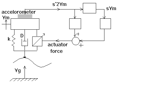
2.A possible active suspension system for AMTRACK trains has been proposed. The system uses a pneumatic actuator in parellel with the passive suspension system, as shown in the figure.

The force of the actuator subtracts from the force applied by the ground, as represented by dispacement, Yg(s). Aacceleration is sensed by an accelerometer, and signals proportional to acceleration and velocity are fed back to the force actuator. The transfer function relating acceleration to groound displacement is
Assume that M=1 and D=K=Cv=2... Ym(s) s^2(Ds+K) ---- = ------------------------- Yg(s) (Ca+M)s^2 + (Cv+D)s +K
Sketch a root locus for this system as Ca varies from zero to infinity.
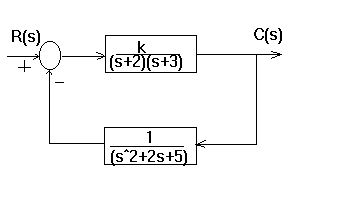
3.For the system shown, do the following

a.Sketch the root locus.
b.Find the jw-axis crossing and the gain,K,at the crossing.
c.Find the gain K, for a damping ratio of 0.2.