State space control of seesaw-cart system

The Seesaw Module shown in our experiment consists of two long arms hinged on to a support fulcrum. The axis is coupled to a potentiometer via a 3:1 gear ratio which is used to measure the angular deflection of the seesaw. The pendulum track and cart (the pendulum itself is not used in this lab and is removed) can easily be placed on top of the seesaw resulting in the experimental setup for this lab. The objective of the experiment is to design a feedback control system that controls the position of the cart such that the seesaw remains horizontal.

By observation, the horizontal equilibrium position is unstable - a small tap in either direction will cause the uncontrolled system to fall over. The goal of your controller, then, is to regulate the system in such a way that the compensated dynamics are stable.

1. State space Model

The nonlinear ordinary differential equations for the seesaw system are shown in the course notes (after the discussion on eigenvalues/eigenvectors). Please review this section to familiarize yourself with the plant. By choosing the equilibrium position to be theta=0, we then linearized the equations about the equilibrium and get the following state-space equations:

     
  .
[ x ]         [ 0       0       1       0 ] [ x ]       [   0   ]  
[ . ]         [                           ] [   ]       [       ]
[ O ]         [ 0       0       0       1 ] [ O ]       [   0   ]
[.. ]   =     [                           ] [ . ]   +   [       ]  V
[ x ]         [-1.45   9.18    -17.2    0 ] [ x ]       [ 3.85  ]
[.. ]         [                           ] [ . ]       [       ]
[ O ]         [10.44   4.38     2.5     0 ] [ O ]       [ -.56  ]       

y= x = [1 0 0 0] X

where the state vector, X, contains the cart displacement (x1 = x), cart velocity (x3 = dx/dt), seesaw angle (x2 = O), and seesaw angular velocity (x4 = dO/dt). Note that here we use O to stand for theta.

         . .
X = [x,O,x,O]' = [x1,x2,x3,x4]' 

is the states of the system (a 4 element column vector) u = V is the input, y is the output. Enter the system matrices under Matlab icon or into a m-file in your matlab directory (call it seesaw.m)

A = [0     0     1      0
     0     0     0      1
    -1.45  9.18  -17.2  0
    10.44  4.38  2.5    0];

B = [0
     0
     3.85
     -0.56];

C = [1   0   0   0];

and run the m-file by typing "seesaw" to the matlab prompt.

One of the first things you might want to do with the state equations is to find the poles of the system; these are the values of s where det(sI - A) = 0, and are exactly the eigenvalues of the A matrix:

poles = eig(A)

Matlab returns

poles =

   2.6918          
  -1.4187 + 0.4619i
  -1.4187 - 0.4619i
 -17.0545          

As you can see, one of them (s1=2.6918) is on the right-half plane, which means that the system is unstable in open-loop.

Matlab can also compute the transfer function of this system:

                        NUM(s)           -1
                H(s) = -------- = C(sI-A)  B + D
                        DEN(s)

using the command

[num,den] = ss2tf(A,B,C,0,1)

returns

num =

         0    0.0000    3.8500    0.0000  -22.0038


den =

    1.0000   17.2000   -2.9300  -98.2860 -102.1902

You could also find the poles of the system using

roots(den)

which returns

ans =

 -17.0545          
   2.6918          
  -1.4187 + 0.4619i
  -1.4187 - 0.4619i

Check to see that this gives you the same answer as before.

2. Controller design

Let's build a controller for this system. The first thing to check is whether the system is controllable. We do this by forming the controllability matrix:

U = [B (A*B) (A^2*B) (A^3*B)]

which returns

U =

   1.0e+04 *

         0    0.0004   -0.0066    0.1128
         0   -0.0001    0.0010   -0.0128
    0.0004   -0.0066    0.1128   -1.9222
   -0.0001    0.0010   -0.0128    0.2171

Then check if it has full-rank (non-zero determinant) by

rank(U)

that returns

ans =

     4

Therefore, it is full rank and the system is controllable, which means we can design a full-state feedback controller to place the closed-loop system's poles at arbitrary positions as we wish. There are several different ways we can approach the problem:

1. By using the method of matching coefficients.

2. Convert the system into control canonical form, choose the control matrix K which would give the desired poles, and then convert back to the original coordinates.

3. Program Ackermann's formula into MatLab.

4. Use the matlab function PLACE.

Before attempting any of these methods, we should decide where we want the closed-loop poles to be. If the criteria for the controller were settling time < 1 sec and overshoot < 5%, then we might try to place the two dominant poles at -5 +/- 5i (at zeta = 0.7 or 45 degrees with sigma = 5 > 4.6). The third and fourth poles we might place at -10 an -20 for starters, and see what the closed-loop behavior is:

p1 = -5 + 5i;
p2 = -5 - 5i;
p3 = -10;
p4= -20;

K = place(A,B,[p1 p2 p3,p4]);

Matlab returns

K =

  197.1387  366.6648   20.9219  103.1236

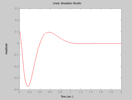
We can simulate the system's response for zero reference input r(t)=0

t = 0:0.01:2;
r = 0*t;
x0 = [0.1  0  0  0];

lsim(A-B*K,B,C,0,r,t,x0);

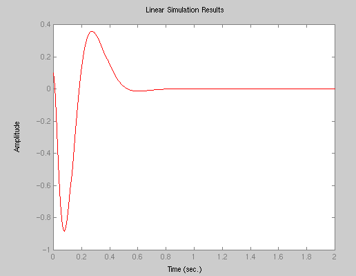
If we wanted a faster response (with the same overshoot), we might place the poles further to the left:

p1 = -10 + 10i;
p2 = -10 - 10i;
p3 = -20;
p4= -30;K = place(A,B,[p1 p2 p3,p4]);

Matlab returns

K =

   1.0e+03 *

    0.9938    3.6049    0.1039    0.6198

Simulate the system's response for zero reference input again

t = 0:0.01:2;
r = 0*t;
x0 = [0.1  0  0  0];

lsim(A-B*K,B,C,0,r,t,x0);

Compare the control effort required (K) in both cases. In general, the farther you move the poles, the more control effort it takes. Since control effort is a measure of the input energy required to control the system, we always want to minimize this parameter!

Pre-Lab:
Do the following calculations before the lab. You will need to turn in your pre-lab results at the start of the lab.

1. Calculate your desired 4th-order pole locations for the following transient
   performance:

       Ts = 0.5s
       %OS = 10%

   Place your non-dominant poles on the real axis at a point 10x further 
   into the left-half plane than your dominant 2nd-order poles.

2. Use the method of "matching coefficients" to derive the state feedback
   vector, Ka = [k1 k2 k3 k4], which will meet the above performance criteria.

3. The state space representation of the system uses units of [m] and [rad]
   for x1, x2, x3, and x4.  However, the experimental system is desinged
   to work with [cm] and [deg].  Convert your state feedback vector, Ka, using
   the following operation:

	K = Ka .* [.01   pi/180   .01   pi/180]

Assignment:

1. Using your state feedback vector, K, determined in the pre-lab, simulate the 
   performance of the system (use MATLAB command LSIM) using u(t)=0, and an 
   initial cart displacement of 0.1cm.  Plot your results, and determine Ts, 
   %OS and damped frequency, wd.

2. Using your experimental data, determine damped frequency, wd.  Compare
   this  with 'wd' obtained from the simulated data and the theoretical one
   from your desired second order poles (the dominant poles). 
   Did the experimental system perform as expected? Note any discrepancies.