 , and
, and  . Make sure you understand this step from Studio #2.
 MatLab's Control Toolbox provides a number of very useful tools for manipulating block diagrams of linear systems. There are three basic configurations that you will run into in typical block diagrams. These are the parallel, series, and feedback configurations. While it is important to feel comfortable calculating the overall transfer function given a complicated block diagram by hand, MatLab is a very useful tool for removing some of the drudgery from this task. In this studio, we will talk about MatLab's functions for automated block diagram manipulation, and also look at how matlab can be used to manually manipulate block diagrams. Using these tools, we will investigate some important properties of feedback systems such as tracking and steady-state error.
	parallel
	series
	feedback
	cloop
	conv
	deconv
To begin this excercise, create two linear systems by typing:
The result should be two transfer functions,
, and
. Make sure you understand this step from Studio #2.
NOTE: This function only works in certain versions of MatLab. type "help parallel" to see if this function is supported on your system.
Consider a diagram with two blocks in parallel, as shown here:

The overall transfer function, C(s)/R(s), is given by T(s) = G1(s) + G2(s). The MatLab function parallel() can be used to determine the overall transfer function of this system. To see how this works, type:
[num, den] = parallel(num1, den1, num2, den2)
The result should be two polynomials which we have placed into the variables `
num'
and `
den'
: These polynomials describe the overall transfer function defined by the
parallel()
operation, i.e. a third-order system: 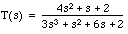
A series connection of transfer functions yields an overall transfer function of T(s) = G1(s) G2(s). The matlab function series() can be used to determine this transfer function. Using the example systems, find the series connection by typing:

[num, den] = series(num1, den1, num2, den2)
As in the parallel connection, the result should be a third-order system: 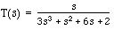
Feedback connections are what the topic of control systems is all about. You should already know that for the following negative feedback connection, the resulting transfer function is given by 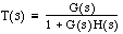 . Rather than simplifying this by hand, T(s) can be found using
MatLab's
feedback()
function.
. Rather than simplifying this by hand, T(s) can be found using
MatLab's
feedback()
function.
[num, den] = feedback(num1, den1, num2, den2, -1)
The result should be: 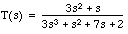 . Note that although MatLab's help file on this function says that
positive feedback is assumed, this is not always the case - negative
feedback is the default in some versions of MatLab. To be sure you are
applying the proper feedback, a fifth arguement (SIGN) must be added
to the function as shown above. If SIGN = 1, positive feedback is used.
If SIGN = -1, negative feedback is used.
. Note that although MatLab's help file on this function says that
positive feedback is assumed, this is not always the case - negative
feedback is the default in some versions of MatLab. To be sure you are
applying the proper feedback, a fifth arguement (SIGN) must be added
to the function as shown above. If SIGN = 1, positive feedback is used.
If SIGN = -1, negative feedback is used.
Another way to produce a feedback system is to use the cloop() function. This function produces the transfer function of a unity-gain feedback system, i.e. the case when G2(s) = 1. If G2(s) = 1, then the feedback connection can be determined as follows:
[num, den] = cloop(num1, den1, -1)
Note that just as with feedback(), cloop() takes a SIGN arguement to specify negative or positive feedback. Unity-gain feedback is very common in control systems, so cloop() is a very useful function to have at your command.
The previous block manipulations could have been done "by hand", instead of using the automated functions, by employing the
conv()
and
deconv()
functions. These functions perform matrix convolution and deconvolution, which is effectively the same thing as polynomial multiplication and division. For example, to multiply  and
and  , simply type:
answer = conv([1 0 1], [1 2 3])
which will result in
answer = [1 2 4 2 3]
, or equivalently 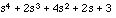 , which is exactly what you get if you were to multiply out these polynomials by hand. Similarly, to divide
answer
by
, which is exactly what you get if you were to multiply out these polynomials by hand. Similarly, to divide
answer
by  , type:
answer2 = deconv([1 2 4 2 3], [1 0 1])
which results in
answer2 = [1 2 3]
, or equivalently  as expected.
conv() and deconv() are very useful tools for many control system analysis and design applications, and you should keep them in mind for when you need to multiply or divide polynomials. They are mentioned here since block reduction is effectively a process of polynomial multiplication, even though the automated functions parallel() , series() , and feedback() are usually more convenient.
G3(s)= s/(s+1)
Consider the following block diagram.
                       -----------
                       |         |
             ----------|  G1     |---------------------|
             |         |---------|                     |
             |  ----                  --------        \|/+
--------------- |G2|------------------|  G3  |-------->O--------
                ----                  --------        +
Sol: This can be reduced to
              ------------------
              |                |
--------------|  G1 + (G2*G3)  |-------------
              |                |
              ------------------
Matlab can be used to give the same result and step response can be plotted
as shown below:
An m-file can be written like this:
NOTE: remember that in Matlab v.4, the "tf" command doesn't work. Instead, series() and parallel() can be called with numerators and denominators, e.g. series(num1, den1, num2, den2).
	num1=1;
	den1=1;
	num2=-1;
	den2=1;
	num3=[1 0];
	den3=[1 1];
	sys1=tf(num1,den1);
	sys2=tf(num2,den2);
	sys3=tf(num3,den3);
	sys4=series(sys2,sys3);
	sys=parallel(sys1,sys4)
	step(sys)
Matlab will respond
Transfer function:
1/(s+1)
and opens a window showing the following plot:

The goal of this studio is to use MatLab to investigate some important features of feedback systems.
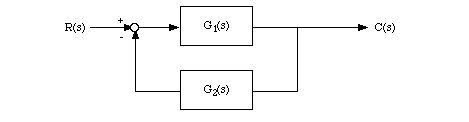
1. Block diagram reduction - write an m-file to find the overall transfer function of the following system, where  ,
and
,
and  :
:
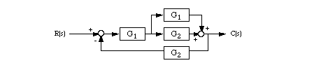
Note that if the version of MatLab you are using does not support the parallel() function, you will need to manually calculate the parallel connection of G1 and G2 in the above diagram. Make sure you simplify the resulting transfer function as much as possible, and print out your results.
Also plot the step response for the transfer function.2.Find the transfer function,T(s) = C(s)/R(s), for the system shown in the figure.
                                              -------
                                  |-----------| s^3 |----------|
                                  |           -------          |
                                - |                            |
                                  |                            |
R(s)  +          ----    +      +\|/   -------       -----     |    C(s)
------->O------->| s |--->O------>O--->| 1/s |------>| 2 |-----|------>
      -/|\ |     -----  +/|\    -/|\   -------   |   -----     |
        |  |              |       |              |             |
        |  |   -----      |       |   -------    |             |
        |  |---| s |------|       |---| s^2 |----|             |
        |      -----                  -------                  |
        |                                                      |
        |                        -------                       |
        |------------------------| s^4 |-----------------------|
                                 -------
3. Feedback - feedback control systems are fundamental requirements for virtually every engineering system.
For example, modern sailboats are equipped with an automatic steering system, in which the captain sets a course,
and the ship's rudder is automatically adjusted by a feedback control system to maintain that course.
The transfer function between rudder position and ship course of a particular 19th century schooner is given
by 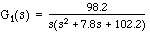 . Unfortunately, automatic control technology was not available when this
ship was commissioned, and
so it does not have automatic steering. During the restoration of this ship, the owners would like to
include a modern control system for automatic steering. Being engineers, and having struggled long and
hard through ENME362, they decide to employ negative feedback to achieve the desired effect. They intend
to measure the actual direction of travel of the ship, c(t), using a GPS system, and subtract this
measurement from the desired ship heading, r(t). A block diagram of the system in the Laplace domain
is shown below:
. Unfortunately, automatic control technology was not available when this
ship was commissioned, and
so it does not have automatic steering. During the restoration of this ship, the owners would like to
include a modern control system for automatic steering. Being engineers, and having struggled long and
hard through ENME362, they decide to employ negative feedback to achieve the desired effect. They intend
to measure the actual direction of travel of the ship, c(t), using a GPS system, and subtract this
measurement from the desired ship heading, r(t). A block diagram of the system in the Laplace domain
is shown below:

a. If this were an open-loop system (no feedback), the captain would turn the wheel to come to a new course, then turn it back to its neutral position when that course was met. If the captain turned the wheel and held it in a non-zero position, the ship would continue turning in a circle. To simulate this effect, apply a step input to the open-loop plant and plot the result.
b. An open-loop automatic system for steering would need a mathematical model of the ship's rudder to estimate how far to turn the wheel, and how long to hold it in its turned position to bring the ship to its new course before retuning the wheel to its zero-position. To simulate this action, use lsim() to produce a plot of the system response for the following input function:

If you don't remember how to use lsim() , go back and look at Studio #2.
c. The open-loop approach to automatic control is very prone to errors due to wind speed, tides, modeling errors, etc. If real automatic steering systems were to use this control approach, cargo ships bound for New York might find themselves in Cuba after several days of open-loop steering. To improve on this situation, let's consider closed-loop control of the system. First, use MatLab to find the closed loop transfer function of the system.
d. Plot the step response of the closed-loop system. Does the feedback work, i.e. does the actual heading track the desired input heading?
e. After implementing the control system, the rudder of the ship is damaged while at sea, causing the rudder transfer function to change to 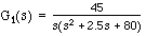 . With this large variation in the parameters of the physical plant, will the automatic steering still work, or will the crew wind up traveling in circles? Plot the time response to a step function for the new closed-loop system. Discuss how the performance of the feedback control system is affected by variations in the plant parameters.
f. With the damaged rudder, what would happen if the open-loop control employed in (b) were used again? Plot the response of the modified open-loop system to the same input F(t) used in (b). Compare the response plot with that of (b). Is the final heading the same as that of (b)? Why or why not? Based on your observations, explain one important reason why a closed-loop control system is vastly preferable to open-loop control.