Studio 2 : Time-Domain Response of First and Second Order Systems

ENME362


Matlab for Controls


MatLab is a wonderful tool for analyzing the time-domain response of systems, both linear and nonlinear. This studio will focus on analyzing the time response of linear systems represented by transfer function models.

Key Commands:

A. Overview of the MatLab Control System Toolbox

MatLab offers a special toolbox for analyzing control systems called (surprise!) the Control System Toolbox. To see the various commands provided by this toolbox, type the command:

A simple demonstration of some of the features of this toolbox can be seen by running the command:

Run this command and you will be rewarded with a number of plots that may not mean much to you yet. That's ok, we'll get there soon.

In version 5 of MatLab, many of the functions in the control toolbox require a special data object called a system, or SYS. A SYS object is an internal MatLab representation of an LTI (linear time invariant) dynamical system. A SYS object may be created in several ways. In this studio we will focus on creating system objects from transfer function polynomials using the tf command.

(NOTE: MATLAB VERSION 5 IS NOT CURRENTLY AVAILABLE IN ENME 362. COMMANDS WHICH REQUIRE A SYS DATA OBJECT CAN BE USED IN MATLAB VERSION 4 BY PASSING (num, den) INSTEAD OF (sys) TO THOSE FUNCTIONS.)

B. Model Creation via tf()

This section only applies to MatLab version 5, since earlier versions do not support the SYS data object.

Recall that transfer functions provide a convenient way of expressing the relationship between the input and output of a linear system when all initial conditions are zero. The roots of the numerator of a transfer function are called the zeros of the system, and the roots of the denominator are called the poles of the system.

Consider a simple mechanical spring-mass-damper system:

Assuming zero initial conditions, a free body diagram of this system results in the following differential equation of motion:

Taking the Laplace transform of this equation and solving for the transfer function X(s) / F(s) results in:

Let's define the numerator and denominator of the transfer function separately (you'll see why soon). The numerator is simply a scalar. At the MatLab prompt, type:

The denominator is a little trickier, since it is a polynomial of the Laplace variable s. In MatLab, a polynomial is represented as a row vector containing the polynomial coefficients in descending order. For example, the polynomial 2s3 + s + 5 would be represented by the vector [2, 0, 1, 5]. For the current problem, the denominator polynomial is 3s2 + 8s + 2. To define the polynomial in MatLab, type:

Now that we have defined the numerator and denominator of the transfer function, a SYS data object for the spring-damper system can be created, using the tf() function. To define the SYS data object for this system (let's call it sys ), type:

MatLab should respond by showing the transfer function of the system. We now have a variable sys which can be used to analyze the spring-mass-damper system. Unfortunately, not all MatLab functions are able to take a SYS object as an argument. For these functions, we will have to describe the system by its numerator and denominator polynomials instead.

Once you have a SYS object, the original numerator and denominator of the system can be recovered using the tfdata() function. Try typing:

MatLab shouold respond by displaying the original numerator and denominator.

C. Poles and zeros

A transfer function can be described by its poles (roots of the denominator) and zeros (roots of the numerator). The roots() function can be used to find the roots of a polynomial. To find the zeros and poles of our example system, type:

Alternately, the zeros and poles may be found simultaneously using the tf2zp() function, where tf2zp stands for "transfer function to zeros & poles". To do this, type:

You should find that zeros and poles are the same as zeros2 and poles2 . In both cases, you should find there are no finite zeros, and the poles are located at s = -2.3874 and s = -0.2792.

Another useful MatLab function, called zp2tf() , can be used to define a transfer function from a set of poles and zeros. In this case, the arguments of the function are the poles and zeros placed in row vector form, and the result of the function is 2 vectors containing the numerator and denominator polynomials. For example, the poles of our example are located at s = -2.3874 and s = -0.2792, and there are no finite zeros. To find the transfer function given this information, type:

Which should return the following:

The third argument of the zp2tf() function is the scalar gain of the transfer function. Why is this needed? Given a set of poles, there are an infinite number of polynomials which have those poles as their roots; if we find one such polynomial, then any scalar multiple of that polynomial will possess the same roots. When you give MatLab a set of zeros and poles, it chooses polynomials for the numerator and denominator which are scaled so that the highest order coefficient of each polynomial is equal to one. In order to produce the desired transfer function, you need to tell MatLab what the scalar gain should be based on this fact. For our example system, a scalar gain of 1/3 is used since, by observation of the original transfer function, we would need to divide both the numerator and denominator through by 3 to produce numerator and denominator polynomials with the highest order coefficient of each polynomial equal to one.

A final way to go between a transfer function representation of a system and a pole/zero representation is to use the poly() function. This is the inverse of the roots() function, but now we provide the roots of a polynomial as arguments to the function (in vector form), and the result of the function is a polynomial which possesses those roots. Just as with zp2tf() , poly( ) returns a polynomial with a highest-order coefficient of one. Using our previously defined variables, type:

These commands will produce the following output:

To produce the original transfer function, a scalar value of 1/3 must be multiplied on the numerator. This is analogous to including the scalar gain of 1/3 to the zp2tf() function.

D. Partial Fraction Expansion and Residues

MatLab can also be used to perform partial fraction expansion of transfer function expressions. This can be very handy for examining the response of individual components of a larger transfer function. First, verify that you still have the original numerator and denominator polynomials, num and den , properly defined. To perform a partial fraction expansion on this transfer function, type:

R is a vector containing the residues, P is a vector containing the component poles, and K is sometimes called the direct term .

The residue() function breaks the transfer function defined by num and den into its n component residues, where n is the order of the denominator:

 
num(s)       R(1)       R(2)             R(n)
------  =  -------- + -------- + ... + -------- + K(s) 
den(s)     s - P(1)   s - P(2)         s - P(n)
If the order of the denominator is larger than the order of the numerator, then K will be zero (can you explain why?)

E. Impulse response

Now that you know how to create SYS data objects and represent systems in terms of transfer functions and poles/zeros, we can look at the time response of linear systems. In this studio we'll consider the response of a linear system to two types of inputs: impulse and step functions.

The impulse response of an LTI system can be plotted using the impulse() function. To try this with our example system, type:

recall that in Matlab v4, you need to replace the 'sys' object with 'num,den', i.e.:

The output should look like:

Note: you won't see the grid lines unless you execute the "grid" command after making the impulse plot

This plot shows the time response of the mass when a unit impulse force is applied to the mass at time t=0s. If you want to see the response for a longer period of time, the impulse() function will also take a time vector as an argument. Try this:

You should get the same basic plot as before, but with a 40s time axis.

Note that instead of using the SYS data object as input to the function, we could also have used the numerator and denominator polynomials, num and den , defined earlier. In general, it is better to stick with using SYS, since some MatLab functions will require this, and future versions of MatLab may require it for all control toolbox functions (get used to it now!).

In some cases, getting a pretty plot isn't enough. Instead, you may want the actual numbers for the mass position as well as the associated time vector. To get this information, type:

Make sure you type the semicolon at the end of the first line, or else the entire output and time vectors will be displayed on the screen. The values describing the position of the mass are now held in x , and the corresponding values of time are held in t .

F. Step response

Step response can be found using MatLab's step() function, which operates the same way as impulse(). In this case, the forcing function is a unit step applied at time t=0s. To plot the step response of our system, type:

or

After typing the plot command, you should see the following:

The x-axis corresponds to the time vector returned by [x, t] = step(sys), and the y-axis shows the response vector, x(t).
If a longer time period is desired in the plot, say t = 0 to 50 sec, you can create the required time vector as:

t = [0 : 0.2: 50];

and then pass this vector to the step() function:

x = step(sys, t)
or
x = step(num, den, t)

G. General linear simulation

A more general technique for simulating the response of a linear system to an arbitrary input signal is the lsim() function. To see how this function works, say we want to simulate the response of our system to a function F(t) = 1 for t<10s, F(t) = 0 for t>10s. First, generate a time vector containing the time points of interest, say for 0 < t < 20s in 0.1s increments:

Next, create an input vector F where the ith element of the vector contains the value of F(ti), and ti is the value contained in the ith element of the time vector:

If you don't fully understand the syntax of setting up the forcing function, don't worry about it too much. With more experience using MatLab this sort of expression will become second nature to you. To plot the response of the system to this input, type:

As you can see, lsim() takes a SYS , input F , and time t as arguments, and returns the output x . This is a very powerful function which allows you to simulate any arbitrary input function you might want to investigate.


Time response: 2nd order systems


In this lab, we will study time responses of control systems. The time response of a control system is usually divided into two parts: the transient response and the steady-state response. We will study these responses for the second order systems. For simplicity, we will mostly use "step input."

Let us look at the following second order (open-loop) system whose transfer function is:


             1           G(s)
      R(s)= ---    _______________
             s     |     b        |   C(s)
      -------------| ------------ |--------->  
                   |s^2 + a s + b |    
                   ---------------

Four typical cases are as follows:
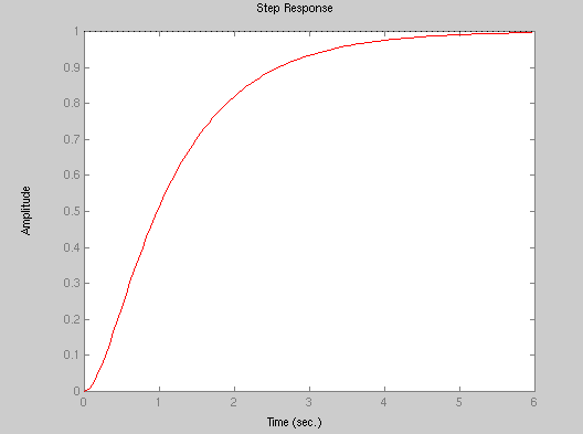
(1) Overdamped

                 4
      G(s) = ------------                (1)
             s^2 + 5 s +4

The step response of system (1) is

(2) Underdamped


                 4
      G(s) = ------------                (2)
             s^2 + s +4

The step response of system (2) is
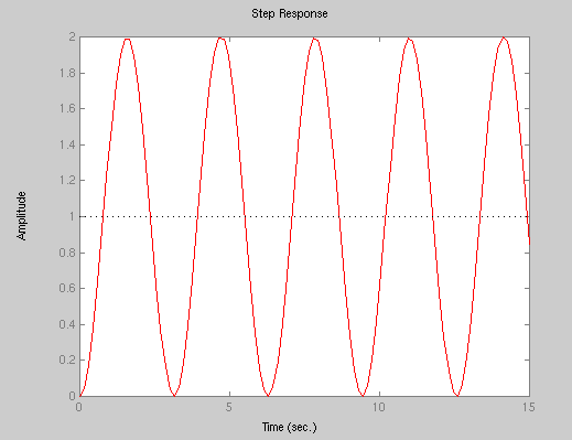
(3) Undamped


                 4
      G(s) = ------------                (3)
              s^2  + 4

The step response of system (3) is

(4) Critically damped


                 4
      G(s) = ------------                (4)
             s^2 +4 s + 4

The step response of system (4) is

Exercise 1: For the above four cases, find the poles and plot the location of the poles in the complex plane by hand, calculate the damping ratio.

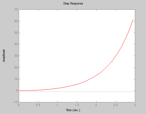
Now let us try another system


                   4
      G(s) = -------------                (5)
              s^2 + s  - 4


The system's step response is

You can see that the system's response diverges and blows up finally, which means the system is "unstable." An unstable system is by no means what we want. What we want is that the system could behave smoothly and have its output follow (track) our desired (reference) input. For this purpose, we use "feedback control". Let us feed the output of the system G(s) back to the input position and compare it with our desired (reference) input to construct the following closed-loop system


                 __         _______       ______
             +  /  \        |     |      |      |   output
  ref input -->(    )------>|  K  |----->| G(s) |--------->           (6)
            r(t)\__/  e(t)  |     | x(t) |      |    |y(t)
                             -----        ------     |
              -  /|\                                 |
                  |                                  |
                  |__________________________________|

The closed-loop transfer function of system (6) is calculated as
                  4 K
     Gc(s) = ------------------                              (7)
              s^2 + s + 4 (K-1)
>From which we can plot the step response as follows: Can you tell why? (It doesn't matter if you can not at this moment.)

Exercise 2: Let K be 0.5, 1.0, 1.5 and 15 respectively, observe and plot the different step responses. Calculate (theoretically) the steady error for the two cases of K=1.5 and K=15, check them against your figure and compare them to see what conclusion you can draw.

Now let us look at the following second order (open-loop) system whose transfer function is:


                 5
    G(s) = ------------                                      (8)
             s (s + 2)

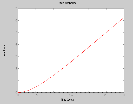
The step response of system (8) is

This system is not asymptotically stable (can you tell why?). Therefore you could not observe a convergent response. This means that we have a system which does not behave as we expected. Now let us use a "feedback control" to regulate its behavior to our desired one. What is our expectation to its behavior or, more precisely, its output? Yes, we wish its output to follow (track) our reference input, say, the step function. Alright, let us use the following unit feedback strategy:


                 __               ______
             +  /  \             |      |   output
  ref input -->(    )----------->| G(s) |--------->          (9)
            r(t)\__/  e(t)       |      |    |y(t)
                                  ------     |
              -  /|\                         |
                  |                          |
                  |__________________________|
                          
                           
Now, you are asked to do the remaining work to fulfill our purpose as defined above.

Exercise 3:
(a) Derive the closed-loop transfer function of system (9).
(b) Do simulation for step response. Calculate (theoretically) the damped natural frequency, peak time, percent overshoot, rise time and settling time and, mark them on your resultant simulation figure.


Assignments

  Do exercises 1, 2 and 3.  

4. Derive the transfer function of the following electrical network. The input is the voltage vi(t) and the output is the voltage vo(t) .

Use the following values of R and C:


5. Write a MatLab m-file which will do the following (turn in m-file and all plots)

a. Calculate and print the poles and zeros of the transfer function

b. Use these poles and zeros to represent the transfer function within MatLab. Don't forget the scaling factor!

c. Re-represent the system in MatLab by entering the numerator and denominator polynomials. Check that the results agree with 5(b).

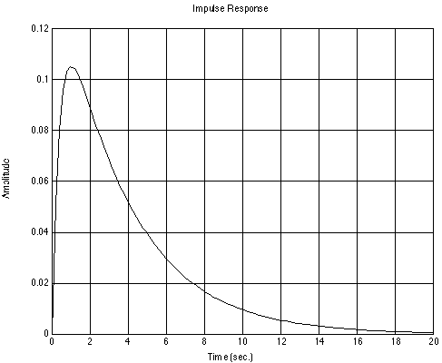
d. Plot the impulse response of the system.

e. Plot the response to an input voltage of vi(t) = 2V, i.e. a scaled step input voltage.

f. Plot the step response of 5(e) when the capacitance is changed from C = 0.4 mF to C = 40.0 mF

g. Use lsim() to plot the response of the original system to an input defined by:

vi(t) = 3V for 0s < t < 9s
vi(t) = 0V for 9s < t


6. Write down (by hand) and turn in the following information:

a. The transfer function of the system.

b. The poles & zeros of the system.

c. The partial fraction representation of the system.

d. Based on the partial fraction representation of the system, what do you expect the impulse response of the system to look like? Why?

e. Describe what happened when C was increased in 5(f). From a physical point of view, try to explain these results.


Studios | Homework | ENME361