Proportional-Integral Controller Design

This experiment employs a cart sliding on a (frictionless? nope...) track. A force is applied to the cart through a DC motor. The input to the system is a voltage, V(t), applied to the motor, and the output of the system is the displacement of the cart, x(t). You will place a unity-gain feedback loop around the plant for position control.

Using the transfer function relating x(t) / V(t), you will investigate the response of the system using the root-locus technique, and also investigate the use of a PI compensator for reducing steady-state error.

System modeling:

In Studio 4, you derived the symbolic expression for the transfer function given in the introduction, i.e.

           X(s)
 G(s) =  -------
           V(s)

The cart was modeled as a simple mass sliding without friction (Of course, this assumption of a frictionless surface is far from true. As you do the experiment, keep this fact in mind!).
The transfer function for the plant (motor + cart) is given by,

Due to modeling uncertainty, the plant gain, Kplant, is not known a priori.

(A) Gain adjustment via root locus:

You will be working with a simple gain controller in the forward path, with unity-gain feedback as shown here:

The root locus for this system looks like:

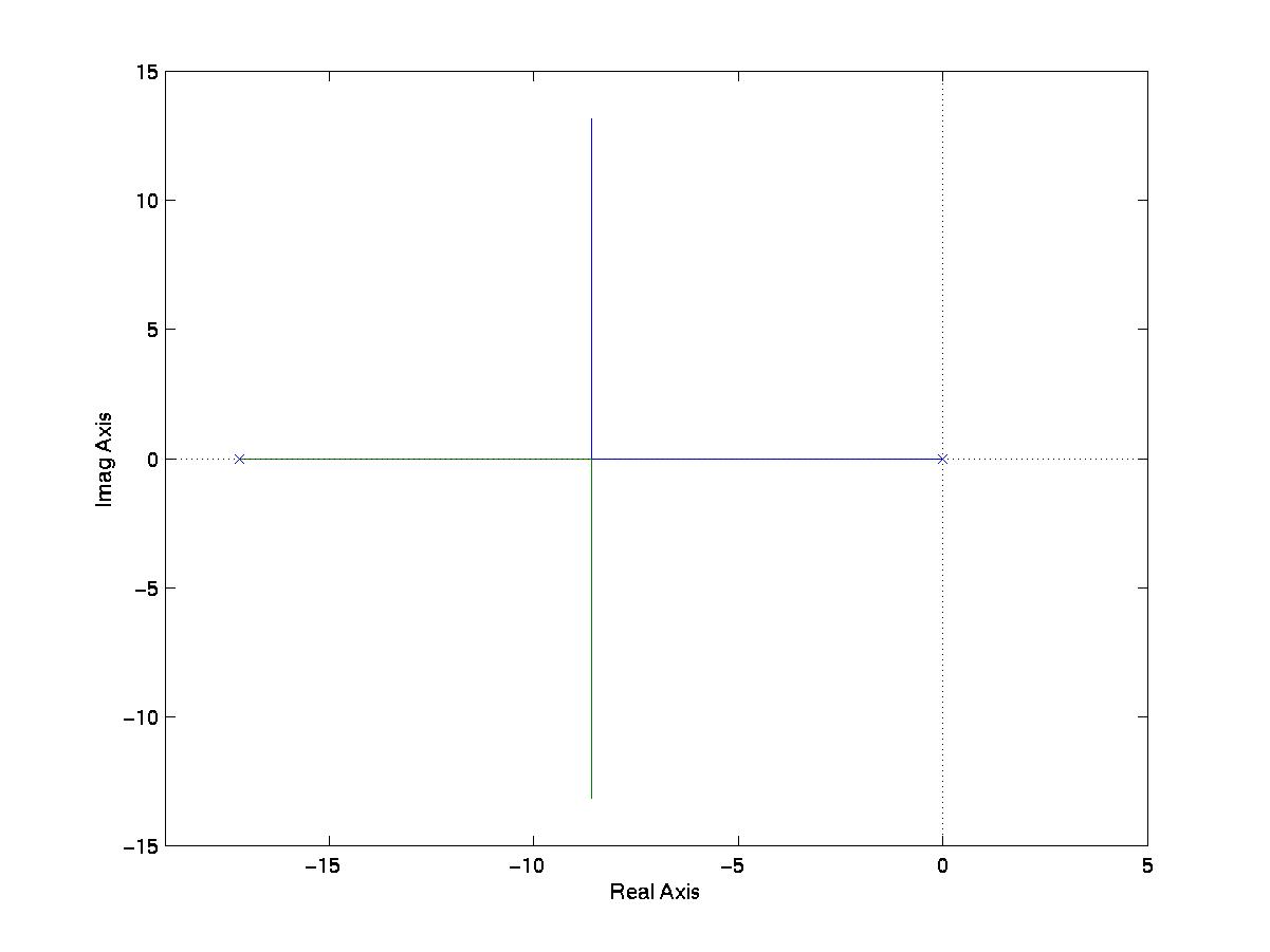
In this section you will experiment with the effects of gain adjustment on system performance.
Do the following:

(1) Place a unity-gain feedback loop around the experimental plant, and 
    implement a simple proportional gain controller, Kp.  
    
    Note that an extra gain of 8 is required in the loop to account for 
    the transfer function between output voltage from the potentiometer 
    to displacement in [cm].

(2) Choose a square wave input, with frequency w=0.2Hz and amplitute A=5cm. 

(3) Run the system for Kp = 0.1, 0.3, 0.5, 0.7, 1.0, 3.0, 5.0.  

    SAVE THE DATA FROM EACH RUN UNDER FILES A3_01.m, A3_03.m, ..., A3_50.m




Assignment:
    A1. Use Matlab to draw the theoretical root locus for the system, and 
        find the value of the total gain, Kp*Kplant, when the system is 
        critically damped ,i.e. when the poles of T(s) meet on the real axis.

    A2. Add your experimental points to the RL plot, and label the value
        of Kp at each point.  To calculate the colsed-loop pole locations 
        for each Kp, use MatLab to measure the damped frequency (wd) or
        the exponential frequency (sigma) from each time-domain plot.

    A3. Use the plot of your experimental data from A2 to estimate the actual 
        value of Kp when the system is critically damped.

    A4. Use the results of A1 and A2 to derive the value of plant gain, Kplant.

    A5. During the experiment, you may have noticed that the steady-state error
        was not approaching zero for small values of Kp even though the 
        system type = 1.  Based on the physical nature of the system, can 
        you explain why this may be so?





(B) PI Control:
In theory, the plant is a type 1 system and should thus yield constant
steady-state error for a ramp input: R(s)=A/s^2 <---> r(t)=At.  In this
section you will implement a PI controller to eliminate the steady-state
error for a ramp input.


The implementation of a cascade PI controller looks like:



To explore the behavior of such a controller, do the following:


(1) Use ramp input (sawtooth), and set A=10cm, w=0.2Hz 

(2) First, run the system without a PI controller to observe the
    steady-state error.  Collect data for proportional gains of
    Kp=0.1, 0.5, 1.0.  

    SAVE THE DATA FROM EACH RUN UNDER FILES NAMED B2_01.m, B2_05.m, B2_10.m

(3) Implement a PI controller:

             s + Zpi
    Gc(s) =  ------ * Kp = Kp + Ki/s     (where Ki = Zpi*Kp)
                s 

    Set Kp=0.5, and collect data for Ki=0.1, 0.5, 1.0.  
    Observe the S.S. errors. Note whether Ess=0 for each case, and 
    how the transient response is affected.

    SAVE THE DATA FROM EACH RUN UNDER FILES NAMED B3_01.m, B3_05.m, B3_10.m




Assignment:
     B1. Derive the expression for Ess without the PI controller.

     B2. Using the value of Kplant found in Assignment A3, and the values 
         of K used in part B(2), compare the theoretical and experimental
         values of Ess.  If your values do not agree, try to explain
         why this may be so.

     B3. Derive the expression for Ess with the PI controller, and show that
         Ess=0 for a ramp input.

     B4. Describe your observations when the PI zero is moved futher into 
         the LHP in terms of Ess and transient response.  Can you explain 
         what is happening?