
In this lab, you will learn the following Matlab commands:
   rlocus           - Calculates and plots the locus of the roots of:
                                        NUM(s)
                        H(s) = 1 + k ----------  =  0
                                        DEN(s)
   rlocfind         - Find the root locus gains for a given set of roots.
   pzmap            - Pole-Zero map of linear systems.
   sgrid            - Plot lines of constant damping ratio
The root locus of a system T(s) is the locus of all possible locations of the closed loop poles as a specified parameter of the system is varied. A common application of the root locus technique is to observe the variation in closed-loop poles as we vary a linear gain element, K, from zero to infinity. Consider the following negative feedback system:
The closed-loop transfer function is
and thus the poles of the closed loop system are those values of s which
satisfy
1+ kG(s)H(s) = 0
As you learned in lecture, this relationship can be used to dserive the magnitude and phase criteria upon which the root locus method is based. Manually sketching the root locus diagram is a valuable skill, since it allows the control system designer to develop the intuition needed to see how changes to the loop transfer function GH(s) will affect the closed loop dynamics. However, accurately sketching the root locus can be time consuming. Matlab offers several powerful tools for plotting and analyzing root locus diagrams. You will learn these tools in this studio.
Consider a plant which has a transfer function of
Make a matlab file called rl.m.
Let's consider what happens when we wrap a unity-gain negative feedback loop
around the plant, and add a gain element the forward path. First, define the loop transfer
function GH(s) in terms of its numerator and denominator:
    numGH = 1;
    denGH = [1 1 4 0];
Now plot the root locus of the system:
rlocus(numGH,denGH)

This plot shows all possible closed-loop pole locations for our pure proportional controller. The plot, however, does not give directions of the loci (what are they?).
Often we want to know the value of the gain, K, which will place the closed-loop poles at a particular set of points on the loci. For example, we may want to find the value of K for which the locus crosses the jw-axis (the point at which the system becomes unstable). Type in the matlab window:
[k,poles] = rlocfind(numGH,denGH)
and then click on the crossing point in the graphics window. Matlab will return to you the locations of all three poles (why three?) as well as the value of K. Try this for a few different points on the locus. Much easier than calculating by hand, yes?
Matlab is a great tool for exploring how the root locus plot for a given system changes as poles and zeros of GH(s) are moved around. For example, consider the following plant:
kGH(s) = k(s+z)/s(s+1)(s+6)
Let's consider what happens for different values of z when 1 < z < 3. First define your system, starting with z = 3:
    z = 3
    numGH = [1 z]
    denGH = conv(conv([1 0], [1 1]), [1 6])
Now plot a series of root loci as z shrinks towards 1:
    for z = 3:-0.2:1
      numGH = [1 z];
      rlocus(numGH, denGH);
      pause
    end
Any surprises? Does the result make sense to you? Could you plot each of the root locus diagrams by hand if needed?
Design Example
Now let's try a typical root locus design example.Given the following loop transfer function kGH(s), pick a value of K that will produce second-order response of T(s) with a settling time of Ts = 4 sec (assume negative feeback is used).
kGH(s) = K/(s+1)(s+3)(s+6)^2
First, recall that settling time for a second-order system is defined by Ts = 4/sigma*xe, and that -sigma*xe is the real part of the dominant second-order poles. Thus, to achieve a settling time of 4 sec, sigma*xe = 1, i.e. the dominant poles must have real parts equal to -1. To find suitable closed-loop pole locations, we will use rlocfind() to graphically select the poles and find the value of K which will put the poles at this point of the locus:
    numGH = 1
    denGH = conv(conv(conv([1 1], [1,3]), [1 6]), [1 6]);
    rlocus(numGH, denGH);
    [k poles] = rlocfind(numGH, denGH)
When you graphically pick your poles with real parts of -1, the result should look like this:
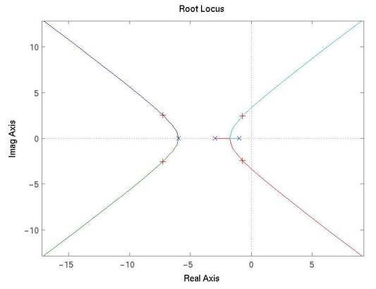
You may need to pick a number of points to get close to a real part of -1. To get an accurate measurement it is also useful to use the zoom function in your plot window to get a higher resolution image near the design point. If you do this carefully, you should be able to find a point similar to:
    selected_point =
       -0.9972 + 2.0011i

    ans =
	   164.4823
So K = 164 will yield the desired settling time of 4 sec.
Note that you should also check that the second-order assumption is valid. When you use rlocfind(), Matlab plots the location of all closed-loop poles for a given value of K. Are the non-dominant poles on the leftmost loci are at least 5x further into the left-half plane than the two dominant poles? If so, you can assume the system will behave approximately like a true second-order system.
To validate your design, plot the time-domain response of the closed loop system. First create the closed-loop system T(s). To do this, assume the feeback is unity gain, and G(s) = GH(s):
    G = tf(164*numGH, denGH)
    H = tf(1, 1)
    T = feedback(G, H)
    step(T)
This code should result in the following time-domain plot:
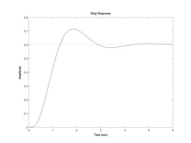
The settling time is defined as the time to reach and stay within 2% of the final steady-state value. Did you meet the performance specification with your controller? Note the locations of the non-dominant poles, which are far enough into the left-half plane compared to the dominant poles to significantly affect the dynamic response.
It is also possible to graphically plot the poles and zeros of a closed-loop system (or any system) without drawing the entire root locus plot by using the pzmap() command. For example, if you wanted to see the location of the poles and zeros of T(s), simply enter pzmap(T) to display the result.
If the above design problem had required finding closed loop poles with a particular damping ratio (or %OS), it would have been a bit more challenging to get the correct answer since the root locus plot does not show lines of constant damping. This is easily corrected using the sgrid command. To see how this works, replot the root locus for the previous example, then apply the sgrid command:
    rlocus(series(G,H))
    sgrid
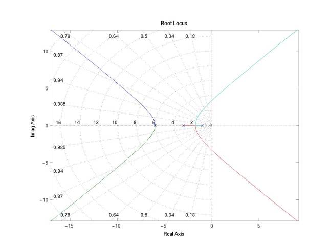
Note that both constant damping and constant natural frequency (NOT damped frequency) lines are displayed in the left-half plane (why not in the right half plane?).
This assignment is essentially similar to your homework assignments, except that you are to use MatLab as an exploratory tool rather than performing detailed calculations.
Given a plant with the following transfer function:
GH(s) = 1/(s+10)(s^2+2s+2)
A proportional-derivitive (PD) controller is added to the forward path of a unity-gain negative feedback loop placed around the plant. The transfer function of the controller is:
    Gpd(s) = K(s-z)
    z = real and negative
(1) Using Matlab, pick the maximum value of z that will make T(s) stable for all values of K.
(2) If z = -8, pick a value of K such that T(s) exhibits second-order behavior with a maximum %OS of 25%.