Unix:
Make a new directory called "matlab" or "me462" or whatever you like (use the "mkdir" command, and then "cd" into that directory). Open up your favorite editor and an xterm; type "tap matlab" in the xterm window, then the command "matlab". Another window should open with a plot in it. This might take a while depending on how many other things are running. Be patient.
Although you can type commands directly into matlab, it is perhaps easiest to put all of the commands that you will need together in an m-file, and just run the file. If you put all of your m-files in the same directory that you run matlab from, then matlab will always find them.PC:
Open up an editor and also run matlab by double clicking on its icon in the Engineering Software subgroup. You can use your favorite editor as long as it produces flat ascii files. The built-in matlab editor or Notepad will work fine. Alternate method: you will for now have to use X-win, a program found under the Internet program group. Once X-win is run, it will connect to a Unix machine and you will be able to log on and proceed as in the Unix side.
In this laboratory, we will practice some fundamentals in MATLAB. The following MATLAB commands will be used. You can use "help topic" to get information for the usage of a specific command.
   diag            - Generate diagonal matrix.
   poly            - Polynomial.
   polyval         - Evaluate polynomial.
   roots           - Find polynomial roots.
   exp             - Exponential.
   det             - Determinant.
   inv             - Matrix inverse.
   rank            - Matrix rank.
   eig             - Eigenvalues and eigenvectors.
   expm            - Matrix exponential.
   plot            - Linear plot.
   title           - Graph title.
   xlabel          - X-axis label.
   ylabel          - Y-axis label.
   print           - Print graph or save graph to file
You may also need to use the following operators and/or symbols:
Char    Name                         HELP topic

   +      Plus                         arith
   -      Minus                        arith
   *      Matrix multiplication        arith
   .*     Array multiplication         arith
   ^      Matrix power                 arith
   .^     Array power                  arith

   \      Backslash or left division   slash
   /      Slash or right division      slash
   ./     Array division               slash

   :      Colon                        colon

   ( )    Parentheses                  paren

   .      Decimal point                punct
   ;      Semicolon                    punct
   %      Comment                      punct
   '      Transpose and quote          punct
   =      Assignment                   punct
or you can try
help matlab/opsto get more infomation. To exit from MATLAB, type quit or exit at the MATLAB prompt, followed by the ``return''key.
a=4/3yields the MATLAB response
a=and assigns to variable a the value of 4 divided by 3.
1.3333
4/3which yields
ans=where ans is a dummy variable that stands for "answer."
1.3333
b=4+7;will create a new variable b whose value is 11, but MATLAB will not display the value of b. However, you can check the value of a variable at any time by entering the variable name at the prompt:
bwhich yields
b=Since a and b have been defined we can do the following:
11
c=a*(b-1)which yields
c=If you are typing in an expression that does not fit on one line, use an ellipsis (three or more periods) at the end of the line and continue typing on the next line, e.g.,
13.3333
p=1+2+...
3+4+6;
Arithmetic operators are the same as those commonly used except that * represents multiplication \ performs left devision, and ^ is the power operator. For the order in which MATLAB performs operations, the power operator ^ has precedence over multiplication * and division / and \, which have precedence over addition + and subtraction -. Precedence of like operators proceeds from left to right, but parentheses can be used affect the order of operation. Try
1+2^3/4*2You should get the results of 5, 2, and 3.3750.
1+2^3/(4*2)
(1+2)^3/(4*2)
MATLAB has several predefined variables such as
i and j stand for square root of -1 which can be used to represent the complex numbers;Try
pi stands for pai;
Inf stands for infinity;
NaN stands for not a number (e.g. 0/0).
c=4/0You should get the results of Inf, NaN, 1.6005+1.2496i, and -0.3642 + 0.0519i.
d=Inf/Inf
y=sqrt(1+4*i)
z=exp(-1+3*j)
>> lab1
>>V1 = [1 2 3]

V1=
    1  2  3
And a column vector V2 can be defined as,
>>V2 = [1; 2; 3]

V2=
    1
    2
    3
As you can see, row elements are separated by spaces (or commas), and column elements are separated by semicolons.
A column vector may be transformed into a row vector, and visa-versa, through
the transpose operation, defined in MATLAB by placing a single quote (') after
the vector definition. For example, the transpose of our column vector V2 is,
>>V2'

ans=

    1  2  3
A Matrix is a series of vectors of like-dimension appended together into a two-dimensional array. Matrices are entered into MATLAB by listing the elements of the matrix and enclosing them within a pair of brackets. Elements of a single row are separated by commas or blanks, and rows are separated by semicolons or carriage returns. For example,
>> A=[1 2; 3 4]yields the MATLAB response
A=

    1  2

    3  4
>> A=[1,2would produce the same result.
3,4]
>> size(A)

ans=

    2  2
>> A(2,2)=5If you add an element to a matrix beyond the existing size of the matrix then MATLAB automatically inserts zeros as needed to maintain a rectangular matrix:
A =
1 2
3 5
>> A(3,3)=6Since a vector is simply a 1 x n or an n x 1 matrix, where n is any positive integer, you can generate vectors in the same way as matrices:
A =
1 2 0
3 5 0
0 0 6
>> v= [sin(pi/3) -7^3 a+1]Alternatively, special vectors can be created using the : operator. The command k=1:10 generates a row vector with elements from 1 to 10 with increment 1. Any other increment can be applied with a second : as follows:
v=
0.8660 -343.0000 2.3333
>> knew = 1:0.25:2To add a row onto matrix A we type
knew =
1.0000 1.2500 1.5000 1.7500 2.0000
>> A = [A;[7 8 9]]To extract the submatrix of A that consists of the first through third columns of the second through fouth rows use vectors as indices as follows:
A =
1 2 0
3 5 0
0 0 6
7 8 9
>> B=A(2:4,1:3)

B =

     3     5     0

     0     0     6

     7     8     9
>> D=diag([1 2 3])

D =
     1     0    0
     0     2    0
     0     0    3
You can create a dummy matrix with all zero elements using the zeros command. This is very useful when you need to create a null matrix which you will fill in element-for-element later.
Z = zeros(2,3)

Z =
     0    0    0
     0    0    0
p=[1 5 6]Zero coefficients must be included to avoid confusion, i.e., q=s^3+5s+6 is entered as
p =
1 5 6
q=[1 0 5 6]A polynomial can be evaluated using the polyval command. For example,
q =
1 0 5 6
>> polyval(p,1)gives the value of the polynomial p at s=1. Using the roots command is a convenient way to find the roots of a polynomial, e.g.,
ans =
12
>> r= roots(p)

r =

    -3

    -2
>> B+DSimilarly, to multiply two matrices do as you would for scalars,
ans =
4 5 0
0 2 6
7 8 12
>> B*DDividing by matrices is also straightforward once you understand how MATLAB interprets the divide symbols (/ and \). Suppose you want to solve for x in the equation P x = Q. To express the solution x=P^{-1}Q in MATLAB use left division as x=P\Q. Now suppose you want to solve y P = Q for y. The solution to this problem is y=Q P^{-1} which you can write in MATLAB using right division as y=Q/P.
ans =
3 10 0
0 0 18
7 16 27
>> R=[4 5

      0 1];

>> S=[2 3

      4 6];

>> R.*S

ans =

     8    15

     0     6
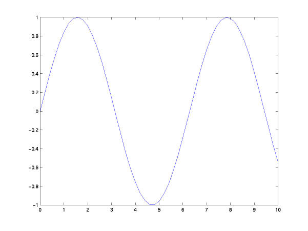
t=0:0.2:10;
y=sin(t);
plot(t,y)
plot(t,y,':')Note that the colon is enclosed in single quotes and separated from the other arguments by a comma. You should get a dotted line. You can make it green (if you have a color monitor) by using
plot(t,y,'g:')
Other options that you might want to try are:Now let's put some useful labels on the plot so someone who looks at it knows what it is. Enter:solid - red r dashed -- green g dotted : blue b dashdot -. white wor tryhelp plotfor more information.
xlabel('Time in seconds');
ylabel('Sin(t)');
title('Sine Wave -- J. Doe, ENME362, LAB1');
To print, you need to know the name of the printer you want to use. This should be posted somewhere near the printer. Just type (within matlab)
print -P<printername>
If you would rather save the plot to print it later (say, you are logged in remotely and don't have a printer handy), then you would typeprint -dps plot.psto save the plot in a postscript format in a file called "plot.ps" (in your current working directory.) Sometime later, you could print it using the command "qpr -q <printername> -ps plot.ps" from a GLUE machine, or if you are using a non-GLUE unix workstation to print, you should instead use the command "lpr -P<printername> plot.ps" since lpr is the standard Unix print service.
To create a batch m-file, you bring up a text editor window where you enter the Matlab commands. There are slightly different things you need to know for each platform.
Macintosh
Windows
Unix
Important:
When working in Windows environment you have to be careful when
saving the m-file. You need to save the m-file in a directory which is in
the path (Try the command [path] at the Matlab command prompt)of
Matlab, otherwise when you try to run the m-file Matlab won't be able to
find it!
diary('diaryfilename')a file called 'diaryfilename'
will be created and all output to your Matlab command window will
be written to this file until you type diary offTo turn the diary back on again while writing to the same file, simply type
diary('diary' by itself simply toggles the diary state).
       (1) Printout of the m-file.
       (2) Printout of the MATLAB results when the m-file is run.
           Use the diary command to save the output to a file,
           then print this file to turn in.
       (3) Printouts of any plots requested.


1. Consider the following matrices and vectors:

              [-5   1   0]         [ 0 ]
          A = [ 0  -2   1]     b = [ 0 ]   c = [-1  1  0]
              [ 0   0   1]         [ 1 ]


(a) Suppose A x = b, find x.

(b) Suppose y A = c, find y.

(c) Let G(s) = c * inv(sI-A) * b, find G(0) and G(1).

(d) Define C_m = [b Ab A^2b], find the rank of C_m.


NOTE: the rank of a matrix is equal to the number of linearly
independent rows or columns in the matrix.  We'll be talking about this
towards the end of the course, but for now you need to know that the
rank of a matrix A is found in MATLAB using the rank() command.
Type 'help rank' for more information.

(e) Now consider an arbitrary nxn matrix A and nx1 vector b.
Let C_m=[b Ab A^2b ... A^{n-1}b]. Write a script file (m-file)
that comuptes the rank of C_m.  Test this program out with several matrices
and vector combinations with varying dimension.

Note: you will need to do some programming to complete this
problem.  The program will need to (1) determine the size of A (=n)
which is also equal to the size of C_m, (2) form C_m (regardless of n),
and (3) find the rank of C_m.  To do this you will probably want to
use a for...next or while loop.  To learn more about the syntax for
these functions, type 'help for' or 'help while'.


2. Consider the function

                n(s)             n(s)=s^3 + 6.4 s^2 + 11.29 s + 6.76
        H(s) = ------   where
                d(s)             d(s)=s^4 + 14 s^3 + 46s^2 +64s + 40


(a) Find n(-12), n(-10), d(-12), d(-10).

(b) Find H(-12), H(-10).

(c) Find all the values of s for which H(s) = 0.
(d) Find all the values of s for which H(s) = inf.
(d) Plot H(s) for s=0 through s=20.  Label your axes appropriately.