Detecting frequencies in a signal
Contents
You need to download an m-file
You first have to download the m-file minabs.m and put it in the same folder as your other m-files.
Sample signal
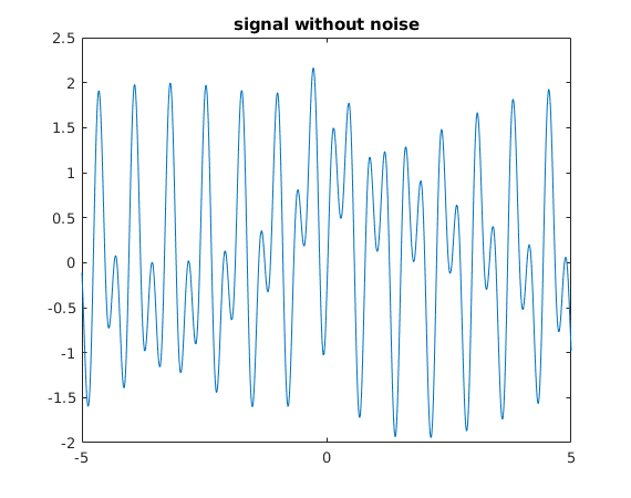
Our sample signal contains two frequencies  and
and  , a nonperiodic part, and noise
rng default;    % reset random number generator so that we get the same results each time

h = .01;
x = -5:.01:5;
N = length(x);

a(1) = sqrt(2); a(2) = exp(1);      % the two frequencies 1.4142 and 2.7183 we want to detect
f = exp(-2*abs(x)) + cos(2*pi*a(1)*x-3) + cos(2*pi*a(2)*x-2);

plot(x,f)
title('signal without noise')
Add random noise
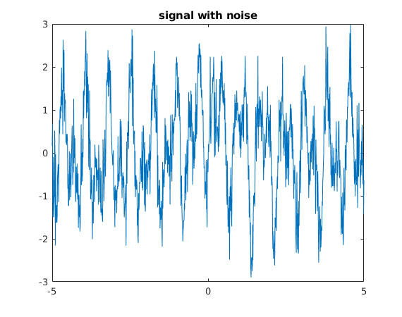
We add some normally distributed white noise.
How accurately can we approximate  and
and  from the noisy signal?
f = f + 0.5*randn(1,N);
plot(x,f)
title('signal with noise')
Method 1: Use autocorrelation
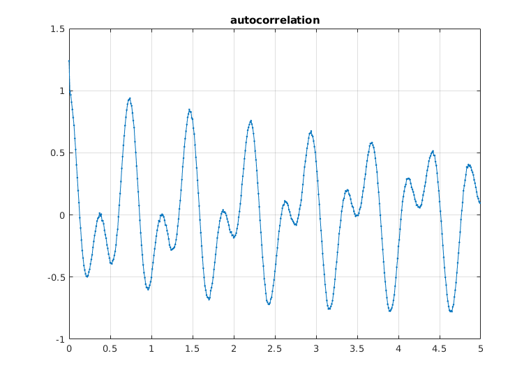
The first relative maximum corresponds to the period  , the second relative maximum to the period
  . Note that we will also relative maxima near integer multiples of
  and
and  .
.
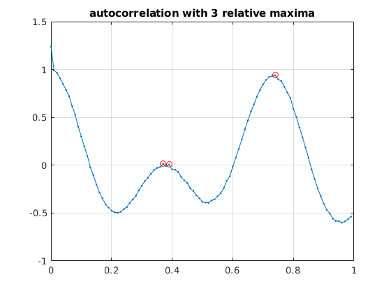
We find the first three relative maxima of the autocorrelation vector using findpeaks. Note that the first and third value seem to correspond to "true relative maxima" whereas the second value seems to be spurious due to the noise in the data.
Therefore we detect the frequencies 2.7027 and 1.3514 (the true values are 2.7183 and 1.4142).
N2 = 2*N;
% F = [f,zeros(1,N)];      % pad with zeros
F = f;                     % without padding (also works)
Fh = four(F);
Gh = abs(Fh).^2;
G = ifour(Gh);             % autocorrelation
xv = (0:N-1)*h;            % entries of G correspond to autocorrelation for 0,h,2h,...

[pks,ind] = findpeaks(G);  % ind are indices of local maxima of vector
lm = ind(1:3);             % first 3 local maxima
periods = xv(lm)           % corresponding x-values give periods
freq = 1./xv(lm)           % corresponding frequencies

error1 = freq(3) - a(1)    % error for freq. a1
error2 = freq(1) - a(2)    % error for freq. a2

figure(1)
plot(xv(1:500),G(1:500),'.-'); grid on
title('autocorrelation')
figure(2)
plot(xv(1:100),G(1:100),'.-',xv(lm),G(lm),'ro'); grid on
title('autocorrelation with 3 relative maxima')
periods =
                      0.37                      0.39                      0.74
freq =
           2.7027027027027          2.56410256410256          1.35135135135135
error1 =
       -0.0628622110217438
error2 =
       -0.0155791257563429
Method 2: Use Discrete Fourier Transform to detect frequencies
We take the Discrete Fourier Transform (DFT) of the data vector (without any padding).
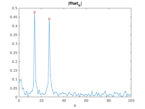
We observe sharp peaks at  ,
,  ,
,  ,
,  .
.
In Matlab we can locate the "peaks" in a vector v using findpeaks:
[pks,ind] = findpeaks(v,'MinPeakProminence',.1,'MinPeakHeight',.2)
finds the values and indices of relative maxima which stand out from their "reference level" by at least .1 and have a height of at least .2. We have to pick the values for MinPeakProminence and MinPeakHeigth carefully so that we capture only the "true peaks" and not the relative maxima from the "noise".
For the DFT the data values correspond to the discrete times 0,1/N,...,(N-1)/N. The k-values correspond to this spacing.
However, our original data  correspond to a spacing of h rather than 1/h. Therefore we have to divide the obtained k-values by N*h to obtain the frequencies.
Here we obtain the frequencies 1.3986 and 2.6973 (the true values are 1.4142 and 2.7183).
fh = four(f);              % Discrete Fourier Transform of signal
v = abs(fh(1:100));
kv = 0:99;
[pks,ind] = findpeaks(v,'MinPeakProminence',.1);  % find relative maxima
                     % which stand out from their "reference level" by at least .1
                     % (use "doc findpeaks" to see the definition of "reference level")
                     % You can also specify 'MinPeakHeight'

kp = kv(ind)         % k-values are frequencies for spacing 1/N
freq = kp/(N*h)      % convert to frequencies for spacing h
errors = freq - a    % errors for frequencies a(1), a(2)

plot(kv,v,'.-',kv(ind),v(ind),'ro')  % plot |fhat_k|, mark detected peaks with red circles
xlabel('k'); title('|fhat_k|')
kp =
    14    27
freq =
           1.3986013986014           2.6973026973027
errors =
       -0.0156121637716966       -0.0209791311563481
More accurate approximations for 1st and 2nd frequency
The first peak for  occurs at
  , which gave us the frequency estimate 1.399 with an error of .015.
If we connect the points  for
for  in the complex plane by two line segments, we can find the closest point to the origin. On this polygonal line the closest point to the origin corresponds to kpeak = 14.14, corresponding the frequency xipeak=kpeak/(N*h)=1.4147. The error for the 1st frequency is now only 4.6e-4 (before it was .015).
We proceed analogously for the 2nd frequency: The second peak for  occurs at
  , which gave us the frequency estimate 2.697 with an error of .02. Using minabs we obtain the improved frequency estimate xipeak=2.719. The error for the 1st frequency is now only 1.1e-3 (before it was .02).
for j=1:2
  K = kp(j)                   % location of j-th peak: K=14 for j=1, K=27 for j=1
  absvals = abs(fh(K:K+2))    % [ |fhat_{K-1}|, |fhat_K|, |fhat_{K+1}| ]
  t = minabs(1./fh(K:K+2))
  kpeak = K + t               % best estimate for location of peak
  xipeak = kpeak/(N*h)        % convert to frequencies for original data at x_j = j*h
  fprintf('error = %e\n',xipeak-a(j))
end
K =
    14
absvals =
        0.0666782093240122         0.476717377011674        0.0916745410923054
t =
         0.160852557431261
kpeak =
          14.1608525574313
xipeak =
          1.41467058515797
error = 4.570228e-04
K =
    27
absvals =
        0.0773635422576332         0.439933703779493         0.125015261384777
t =
         0.221285136319633
kpeak =
          27.2212851363196
xipeak =
          2.71940910452744
error = 1.127276e-03