Detecting frequencies contained in a discrete signal using the FFT

You need to download some m-files
Define f(x) and find Fourier transform fhat(xi)
Take samples g_j = f(jh) for j=-M...M
Find discrete Fourier transform
How is qhat related to fhat?

You need to download some m-files

Download the following m-files and put them in the same directory with your other m-files:

four.m , ifour.m , Four.m , iFour.m

format compact        % don't print blank lines between results

Define f(x) and find Fourier transform fhat(xi)

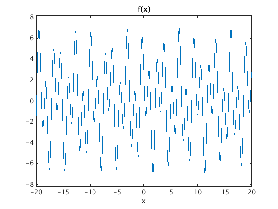
Here we define a signal which contains frequencies 0.31 and 0.73, and some smooth decaying function.

Note that the Fourier transforms contains delta functions concentrated at xi=.31, xi=-.31, xi=.73, xi=-.73.

syms x xi                                    % set up symbolic variables
Pi = sym('pi');                              % and symbolic pi
                                             % signal which contains frequencies 0.31 and 0.73
f = 3*cos(0.31*2*Pi*x)-4*sin(0.73*2*Pi*x)+x*exp(-Pi*x^2);
fhat = simple(Four(f,x,xi))                  % find Fourier transform and simplify

ezplot(f,[-20,20]); title('f(x)')   % plot f

fhat =
(3*dirac(xi - 31/100))/2 + (3*dirac(xi + 31/100))/2 + dirac(xi - 73/100)*2*i - dirac(xi + 73/100)*2*i - xi*exp(-pi*xi^2)*i

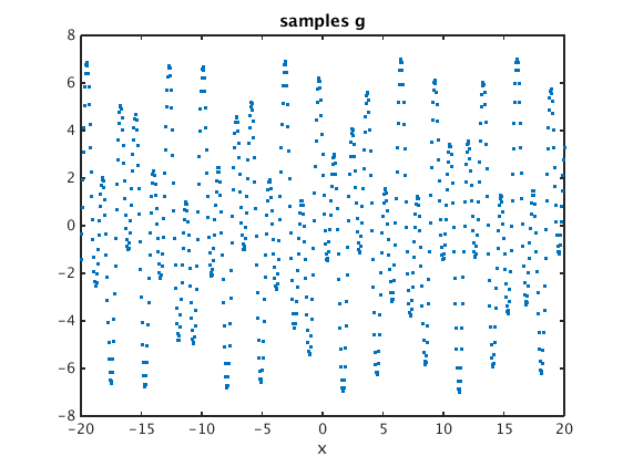
Take samples g_j = f(jh) for j=-M...M

h = 0.05;                                    % spacing
M = 400;
N = 2*M+1;                                   % number of values
X = (-M:M)*h;                                % discrete x values

g = double(subs(f,x,X));                     % samples of f
plot(X,g,'.')                                % plot samples
xlabel('x'); title('samples g')

Find discrete Fourier transform

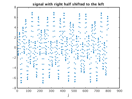
gs = ifftshift(g);                           % shift left half of signal to the right
figure(1); plot(gs,'.');
xlabel('j'); title('signal with right half shifted to the left')

qhat = four(gs);
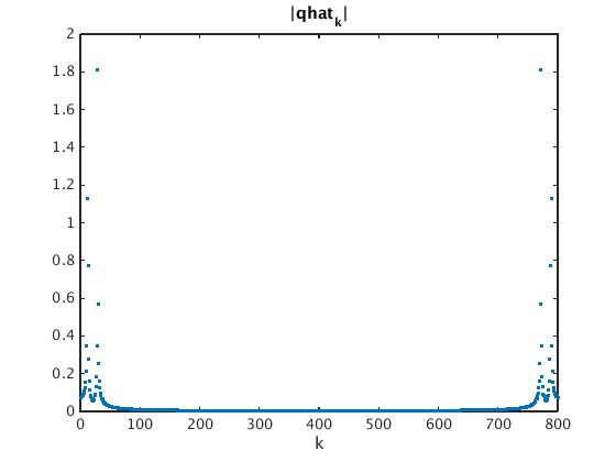
figure(2); plot(0:N-1,abs(qhat),'.');
xlabel('k'); title('|qhat_k|')

qhats = fftshift(qhat);                      % shift right half to the left
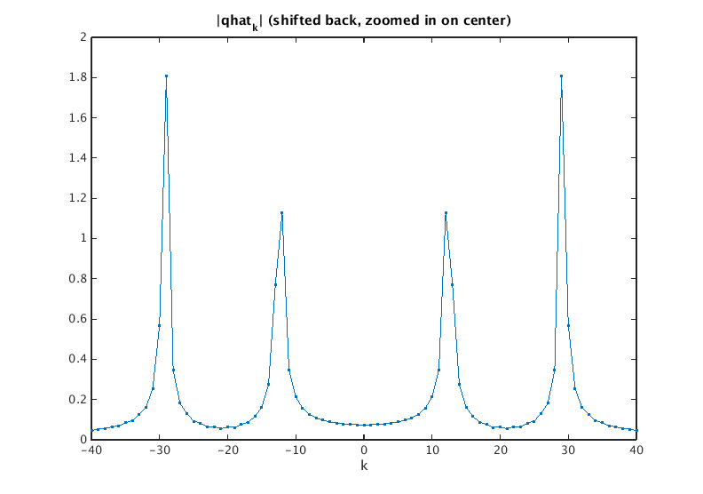
figure(3); plot(-M:M,abs(qhats),'.-');
xlim([-40 40]); xlabel('k')                  % show -40...40 on horizontal axis
title('|qhat_k| (shifted back, zoomed in on center)')

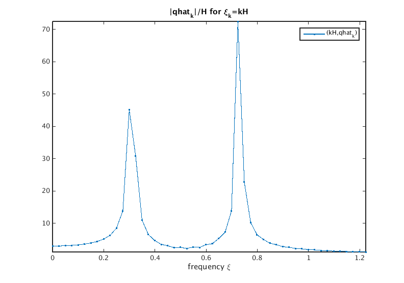
How is qhat related to fhat?

Answer: for H = 1/(N*h) we have that qhat_k/H approximates fhat(k*H).

Note that we see peaks near xi=0.2996 and xi=0.7241. This allows us to detect the frequencies contained in the discrete signal.

H = 1/(N*h);                                 % spacing in frequency domain

disp('    xi_k     |qhat_k|')                % print table of xi_k and |qhat_k|
disp([(0:34)'*H, abs(qhat(1:35))'])

plot((0:49)*H,abs(qhat(1:50))/H,'.-');       % plot points (k*H,|qhat_k|/H)
axis tight
title('|qhat_k|/H for \xi_k=kH')
xlabel('frequency \xi'); legend('(kH,qhat_k)')