Examples for discrete Fourier transform

Contents

You need to download some f-files

Download the following m-files and put them in the same directory with your other m-files:

format compact        % don't print blank lines between results

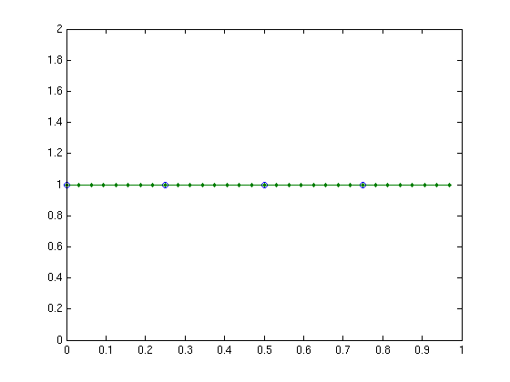
Example 1

Here all data values are 1, so the interpolating function ftilde(x) should be the constant function 1, corresponding to fhat=[1,0,0,0].

f = [1,1,1,1]
fhat = four(f)

f =
     1     1     1     1
fhat =
     1     0     0     0

Plotting the interpolating function

We find a Fourier vector ghat of length 32 which corresponds to the SAME function ftilde(x) by sticking zeros into the middle of the vector. Then the inverse Fourier transform of ghat gives the values in the time domain, but now on a finer grid.

N = 4;
x = (0:N-1)/N;        % grid points
Np = 32;              % use grid with Np=32 for plotting
xp = (0:Np-1)/Np;     % grid points
ghat = fext(fhat,Np)  % extend Fourier vector to length 32 by sticking 0's in middle
g = ifour(ghat);      % values of interpolating function on fine grid
plot(x,f,'o',xp,g,'.-')

ghat =
  Columns 1 through 13
     1     0     0     0     0     0     0     0     0     0     0     0     0
  Columns 14 through 26
     0     0     0     0     0     0     0     0     0     0     0     0     0
  Columns 27 through 32
     0     0     0     0     0     0

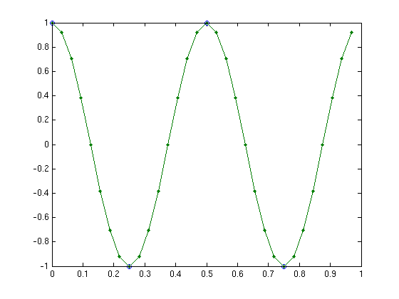
Example 2

Here the interpolating function should be the function cos(4*pi*x), corresponding to fhat=[0,0,1,0].

f = [1,-1,1,-1]
fhat = four(f)

f =
     1    -1     1    -1
fhat =
     0     0     1     0

Plotting the interpolating function

In order to obtain ghat which represents the SAME function ftilde(x) we need to split the coefficient 1 into 1/2 for frequency 2 and 1/2 for frequency -2:

ghat = fext(fhat,Np)  % extend Fourier vector to length 32 by sticking 0's in middle
g = ifour(ghat);      % values of interpolating function on fine grid
plot(x,f,'o',xp,g,'.-')

ghat =
  Columns 1 through 7
         0         0    0.5000         0         0         0         0
  Columns 8 through 14
         0         0         0         0         0         0         0
  Columns 15 through 21
         0         0         0         0         0         0         0
  Columns 22 through 28
         0         0         0         0         0         0         0
  Columns 29 through 32
         0         0    0.5000         0

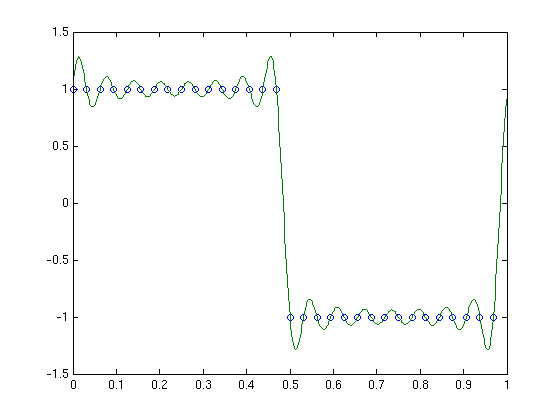
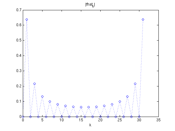
Example 3

Here is a signal which is first 1 and then -1. Note that

f = [ones(1,16),-ones(1,16)]
fhat = four(f);
N = length(f); x = (0:N-1)/N;
plot(0:N-1,abs(fhat),'o:'); xlabel('k'); title('|fhat_k|')

f =
  Columns 1 through 13
     1     1     1     1     1     1     1     1     1     1     1     1     1
  Columns 14 through 26
     1     1     1    -1    -1    -1    -1    -1    -1    -1    -1    -1    -1
  Columns 27 through 32
    -1    -1    -1    -1    -1    -1

Plotting the interpolating function

Np = 512; xp = (0:Np-1)/Np;
ghat = fext(fhat,Np); % extend Fourier vector to length 512 by sticking 0's in middle
g = ifour(ghat);      % values of interpolating function on fine grid
plot(x,f,'o',xp,g)

Published with MATLAB® R2014a