Motion in earth's gravity

Law of gravity
Newton's law
Rewriting the problem as a first order ODE system
Low initial speed
Medium initial speed
High initial speed

Law of gravity

Assume the center of the earth is at the origin, and a spacecraft has position y=(y1,y2) at time t. Then the force from gravity is directed at the earth, and the magnitude is proportional to 1/d^2 where d is the distance to the center of the earth.

Hence the force vector is -C*y/||y||^3 = -C*y/(y1^2+y2^2)^1.5

Newton's law

Newton's law states that mass*acceleration is the sum of all forces acting on the mass.

If the spacecraft has position (y1(t),y2(t)) at time t, the acceleration vector is (y1''(t),y2''(t)).

Hence the functions y1(t), y2(t) satisfy the following system of ODEs:

y1'' = -c*y1/(y1^2+y2^2)^1.5
y2'' = -c*y2/(y1^2+y2^2)^1.5

We will use c=1 for simplicity from now on.

This is a system of 2nd order ODEs. We need an initial condition for the initial position and for the initial velocity: E.g., assume we are a distance of 2 from the origin, and have an initial speed of 0.95 in tangential direction:

(y1(0),y2(0)) = (0,2) , (y1'(0),y2'(0)) = (0.95,0)

Rewriting the problem as a first order ODE system

We introduce additional functions y3(t):=y1'(t) and y4(t):=y2'(t).

Now we obtain the following first order ODE system for y1(t),y2(t),y3(t),y4(t):

y1' = y3
y2' = y4
y3' = -y1/(y1^2+y2^2)^1.5
y4' = -y2/(y1^2+y2^2)^1.5

We can therefore write the ODE system as y' = f(t,y) with the following function f(t,y):

f = @(t,y) [ y(3); y(4); -y(1)/(y(1)^2+y(2)^2)^1.5; -y(2)/(y(1)^2+y(2)^2)^1.5 ];

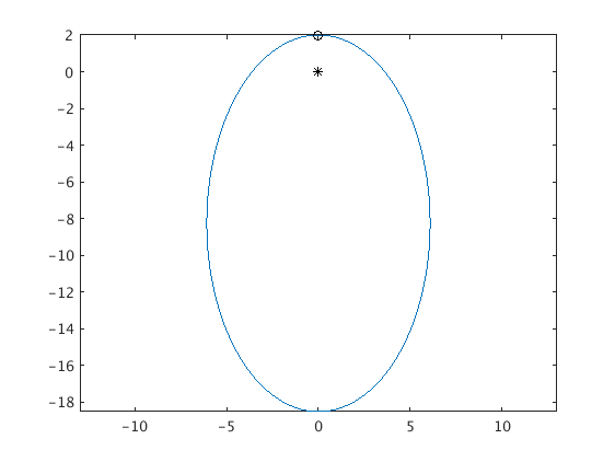
Low initial speed

First we use an initial speed of v=0.95. The solution is periodic in time, and the trajectory is an ellipse where one of the foci is the center of the earth.

opt = odeset('RelTol',1e-10,'AbsTol',1e-10);   % use higher accuracy for ode45
[ts,ys] = ode45(f,[0 300],[0;2;0.95;0],opt);
plot(ys(:,1),ys(:,2)); axis equal; hold on     % plot trajectory in the (y1,y2) plane
plot(0,0,'k*',0,2,'ko')                        % mark the center of earth with '*'
                                               % and the initial point with 'o'

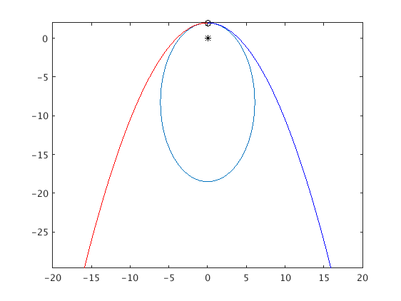
Medium initial speed

Now we use an initial speed of v=1. The trajectory is a parabola where the focus is the center of the earth.

We first solve the ODE for t going from 0 to 100 and plot this in blue.

Then we solve the ODE backward in time, with t going from 0 to -100 and plot this in red.

v = 1;
[ts,ys] = ode45(f,[0 100],[0;2;v;0],opt);      % Solve ODE for t=0...100
plot(ys(:,1),ys(:,2),'b');
[ts,ys] = ode45(f,[0 -100],[0;2;v;0],opt);     % Solve ODE backwards for t=0...-100
plot(ys(:,1),ys(:,2),'r');

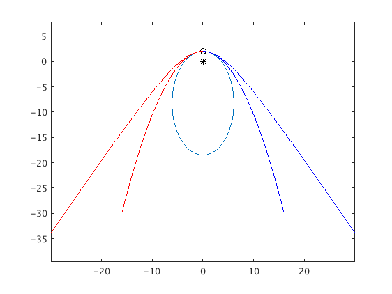
High initial speed

Now we use an initial speed of v=1.05. The trajectory is a hyperbola where one of the foci is the center of the earth.

Again, the solution for t from -100 to 0 is shown in red, and for t from 0 to 100 is shown in blue.

v = 1.05;
[ts,ys] = ode45(f,[0 100],[0;2;v;0],opt);
plot(ys(:,1),ys(:,2),'b');
[ts,ys] = ode45(f,[0 -100],[0;2;v;0],opt);
plot(ys(:,1),ys(:,2),'r');
hold off