Patch Foraging With Memory and learning
E. Gurarie, M. Auger-Méthé, J. Merkle, C. Gros, more…
May 5, 2019
1 Background
Following the BIRS-Banff workshop on Animal Movement and Learning, we propose developing a model to explore how learning might be important in a “stationary” state - i.e. where updating a dynamic world model based on experiences can help inform decisionts - vs. a “transient” state where a novel environment is introduced into the world. Importantly, the model is meant to be useful for exploring actual data.
This model will contain (a) a flexible model of a world consisting of discrete “habitat types” with unique consumption/regeneration dynamics, such that a variety of real habitats can be approximated, (b) a memory / learning model that updates habitat preferences (in a Bayesian way) based on experiences, can accomodate new habitat types, and has a spatial component and forgetting dynamics, (c) a movement model that is similar to a step-selection framework, with coeffecients for specific habitat types obtained from the memory/learning model, (d) clear measures of performance.
One of the main purposes of this model will be to explore the conditions under which a certain extent of behavioral plasticity / openness to novelty / exploratory instinct can be beneficial or detrimental.
Roughly, the schematic of the model is summarized in the crude cartoon below, where the left two panels indicate a dynamic learning about a fixed environment with depletion/regeneration dynamics, and the right panel indicates the end result of a new environmental element (in this case - a road) being introduced. 
2 Model
2.1 World properties
The world consists of \(n\) patches among which an individual moves in discrete time, i,e,~\(Z_t \in \{1,2 ..., n\}\). There are \(k\) types of patches (\(j \in \{1,2, ... k\}\)), which are characterized by unique intrinsic qualities (\(Q_{max,k}\)). Optionally, we can include a type-specific rate of regeneration (\(r_j \in [0,1]\)) and consumption rate \(c_j\). Thus, given the vector of true qualities at time \(t\) \(Q_{i,t}\):
\[ Q_{i,t+1} = \begin{cases} Q_{i,t} (1 - c) & \textrm{if}\,\, Z_t = i\\ Q_{i,t} + r_i \, (Q_{max,i} - Q_i) & \textrm{else}\\ \end{cases} \]
If \(c\) and \(r\) are equal to 0, then the qualities are constant. Otherwise, the quality of a patch decreases exponentially as long as it is occupied by the animal, and increases exponentially to its maximum quality when the animal is absent. The quality is easiest to think of as actual forage availability, but may also combine a risk of predation, which also increases the longer one stays in a patch.
In a non-consumptive model, a simple measure of performance is the average quality of the visited patches \(\overline{Q}\). In the consumption/regenerating model has the advantage of leading to a more subtle measure - the total (or average) consumption of the animal over a track, i.e.
\(C = \sum_{t = 1}^{t_{max}} c \, Q_{Z_t, t}\)
In the figure below, we simulate a 20 patch world with two qualities of habitat (one high, but with rapid depletion and slow regeneration, the other low, but with low depletion and rapid regenaration), and illustrate the quality time-series for each patch as an individual marches through each one.
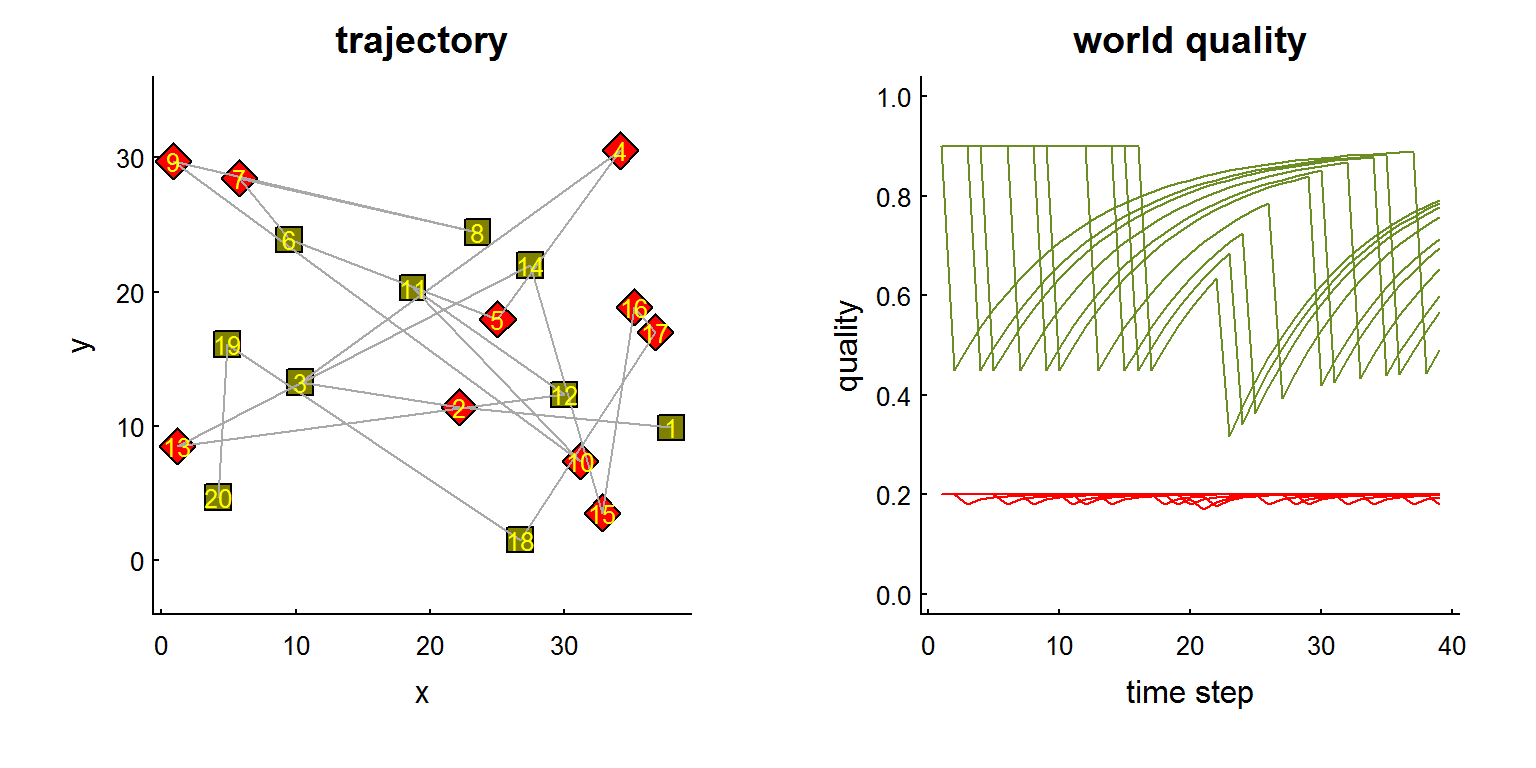
Figure 1. Left: Schematic of 20 patch world where red and green patches indicate lower (0.2) and higher (0.9) intrisic quality patches, respectively. Grey lines indicate a trajectory that moves, simply, from 1 to 20 and back to 1. Right: quality of visited locations with consumption and regeneration rates of 0.5 and 0.1 for the higher-quality patches, which deplete quickly and recover slowly, and 0.1 and 0.5, respectively for the lower-quality habitats, which deplete slowly and recover quickly.
2.2 Basic Movement models
2.2.1 Well-informed movement: no learning or memory
A straightforward model of movement among patches selects the best available patch while discounting for distance, i.e. the probability of moving from patch \(i\) to \(j\) is given by:
\[Pr(Z_{t+1} = z_j\,|\,Z_t = z_i) \propto Q_j \exp({-d_{ij}/\delta)}\]
where \(Q_j\) is the quality (later - remembered) of site \(j\), \(d_{ij}\) is the distance between locations \(i\) and \(j\), and \(\delta\) is the discounting for distance, which encompasses the “cost” of moving between patches. At the limit \(\delta \to 0\), the walker never leaves it spot; if \(\delta\) approaches infinity, the transition probabilities are exactly proportional to quality, whether near or far. This matrix is normalized across the rows to make it a transition matrix.
In the non-comsumptive version, this is a Markov transition probability matrix, and it is (probably straightfoward) to show that the stationary state is proportional to the quality of the landscape types, depending perhaps on the distribution of distances among the types. In the consumptive-regenerative version (\(c\) and \(r > 0\)), the process is dynamic because \(Q_j\) depends on previous visits, and the matrix itself is not Markovian. However, this process does attain a stationary state. Note that this formulation also makes staying quite likely.
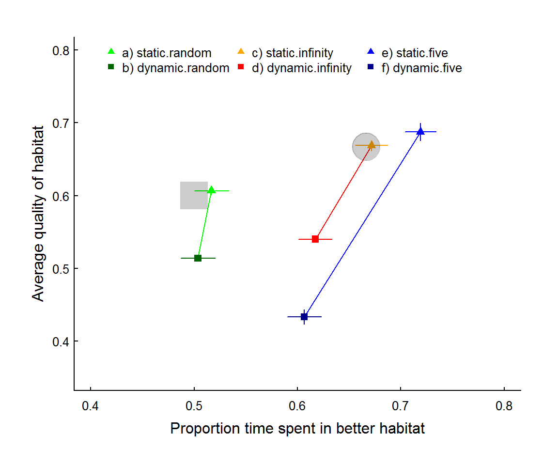
Figure 2: Average intrinsic quality of visited patch against proportion time in better habitat across 6 simulation scenarios with 10 patches each of quality 0.4 and 0.8 (30 worlds x 150 simulation steps, removing first 50 to remove transient state where needed). The six scenarios are: (a,b) random movement; (c,d) informed movement with no distance attenuation (\(\delta \to \infty\)); and (e,f) local jumping (\(\delta = 5\)). In all pairs (connected with lines) the lighter triangles and darker squares represent static and dynamic (i.e. with consumption + regeneration) patch qualities, respectively. The grey square represents the expectation for the random movement model (P=0.5, Q.mean = 0.6) and the grey circle represents the expectation of the ideal free distribution - aka optimal foraging - (P = 2/3, Q.mean = 2/3).
From figure 2 - as expected - informed movement improves foraging over random (green points compared to others), and dynamic landscapes (obviously) lowers the average quality of visited patches. Interestingly, in the static environments, distance attenuation tends to increase the proportion spent in better habitat as the indiviudal becomes more locally “conservative” and hangs out in patches (or regions of patches) with higher quality. In the dynamic case, in contrast, local depletion leads to lower quality and proportion time spent - i.e. the local conservatism of movement means that disproportionate amount of time is spent in poorer quality patches.
2.3 (Proposed) learning and memory model
A proposed (simple) model of memory and learning in this scenario is described as follows:
World model: A discrete “world model” (\(\widehat{T_i}\)) is retained by the individual as it moves. The model knows the locations of all possible patches, but is not aware of the categorical type until it visits each patch, thus each patch is (in a 2-type scenario) is either type A, B, or U (unknown). Once an animal has visited all patches its categorical knowledge is perfect. The animal also retains a “baseline expectation” \(\overline{Q}\), the average \(Q\) experienced from its movements. An important tweak to the world model: The animal might also “forget” what patches might be after a long enough time, i.e. some known types might revert to U at some fixed rate.
Movement rules: At each time-step, the individual weighs going to any particular patch according to a simple step-selection type rule, where: \[Pr(Z_{t+1} = z_j\,|\,Z_t = z_i) \propto \widetilde{\beta_{T_j}} \exp({-d_{ij}/\delta)}\] Where the \(\widetilde{\beta_{T_j}}\) is the median of an absolute preference distribution for each type of habitat (for simplicity, constrained between 0 and 1 for each type). An animal that is very conservative will have a very low preference for heading to an unknown patch (\(\beta_U \ll \{\beta_A, \beta_B\}\)). Generally, animals should scale their preference for the better habitat in proportion to the amount by which it is better, though depletion and regeneration will lower that proportion respectively.
Updating rules: The overall goal of a learning mover is to obtained a learned, optimized posterior estimate for the \(\beta\)’s for the known types. In one simple process, an animal might begin with a Unif(0,1) prior for each type. Each time it visits patch \(i\) of type \(j\), it compares the \(Q_i\) to its baseline expectation \(\overline{Q}\). If \(Q_i > \overline{Q}\), then the visit is considered a “success”, and the uniform distribution for \(\beta_j\) is updated to a Beta(2,1) distribution (mean 2/3). If it is worse, the distribution is updated to a Beta(1,2) (mean 1/2), and so on. Thus after \(n\) visits to patches of type \(j\), the posterior distribution is simply Beta(a+1,n-a+1), where \(a = n_{Q_i>\overline{Q_i}}\) is simply the count of times that the visited patch was better than the running mean. These updating rules would constitute a clear learning process. I’m not sure if this is an optimal algorithm!? But it has the advantage of being intuitive and simple.
Exploration/forgetting parameter: The \(\beta_U\) should be different from the other parameters in that it is fixed. Similarly, in the world model, it might be interesting to explore how the rate of “forgetting” might affect the (stationary) dynamics of this process. These are both good ways to characterize “opennenss to novelty” or “behavioral plasticity”. A question: under what conditions is it beneficial to be more or less exploratory? Presumably, in a more static, well-explored environment, there is little benefit to exploring new territories or forgetting their types. In a dynamic environment - or in a transient (perturbed) world state - these are both presumably more valuable.
Major perturbation: Should an absolutely new type of habitat appear (e.g. a forest fire or a major development), this would be modeled by a bunch of patches becoming of a new type (e.g. Type C), but otherwise this would have relatively little impact on the functioning of the model. A new \(\beta\) would be introduced into the movement rules, with an uninformed prior, which then gets updated as needed. In this way, both dynamic stationary states (e.g. with habitats switching), and transient states can be explored with the same framework.