 Plane Stress Analysis of Cantilever Beam
 Plane Stress Analysis of Cantilever Beam
[ Problem Statement ]
[ Finite Element Mesh ]
[ Displacements ]
[ Stress Contours ]
[ Input/Output Files ]
You will need Aladdin 2.0 to run this problem.
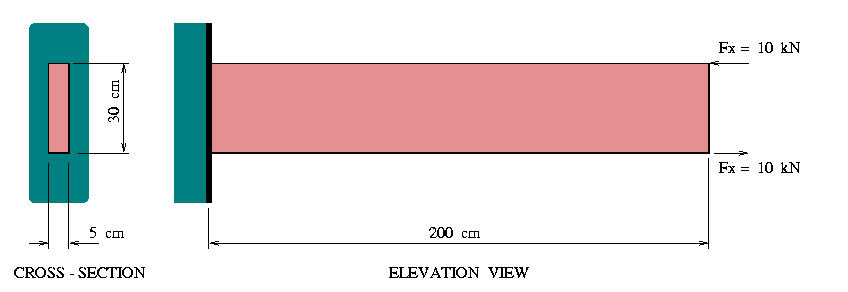
Figure 1 shows an elevation and cross section view of a cantilever beam subject to an end moment couple of 10 kN forces spaced at 30 cm centers.

The cantilever is 200 cm long, 30 cm high, and 5 cm thick, and is attached to a wall with full fixity (i.e., no rotations allowed). It is constructed from a material having Young's modulus E = 20000000 kN/m^2 and Poisson's ratio = 1/3.
This example presents a finite element analysis of the cantilever beam assuming plane-stress behavior. We will:
Finite Element Mesh
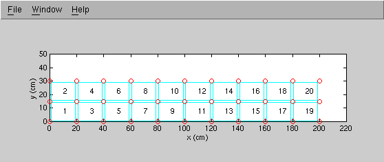
Figure 2 is a MATLAB plot of the finite element mesh.

The block of Aladdin code:
    beam_length  =  200 cm;
    beam_width   =    5 cm;
    beam_height  =   30 cm;

    node = 0;
    x = 0 cm ; y = 0 cm;
    while(x <= beam_length) {
        node = node + 1;
        AddNode(node, [x, y]);

        y    = y + beam_height/2;
        node = node + 1;
        AddNode(node, [x, y]);

        y    = y + beam_height/2;
        node = node + 1;
        AddNode(node, [x, y]);

        x = x + beam_length/10;
        y = y - beam_height;
    }
creates a rectangular block of 33 nodes beginning at (x,y) = (0 cm, 0 cm) and finishing at (x,y) = (100 cm, 30 cm). The block of code:
    i = 1; elmtno = 1;
    while(elmtno <= 19) {
      AddElmt( elmtno, [   i, i+3, i+4, i+1 ], "cantilever_elmt_attr");
      elmtno = elmtno + 1;

      AddElmt( elmtno, [ i+1, i+4, i+5, i+2 ], "cantilever_elmt_attr");
      elmtno = elmtno + 1;
      i = i + 3;
    }
systematically attaches twenty plane-stress/plain-strain finite elements to the nodes.
Section and Material Properties
The section and material properties are:
    ElementAttr("cantilever_elmt_attr") { type     = "PLANE_STRESS";
                                          section  = "cantilever_section";
                                          material = "cantilever_material"; }

    SectionAttr("cantilever_section") { depth = beam_height;
                                        width = beam_width; }

    MaterialAttr("cantilever_material") { poisson = 1.0/3.0;
                                          E       = 20000000 kN/m^2; }
Boundary Conditions
We assume that at its base the cantilever is fully-fixed in the horizontal direction. Node 1 is also fixed in the y-direction. Nodes 2 and 3, however, are allowed to displace in the vertical direction i.e.,
    FixNode( 1, [1,1] );
    FixNode( 2, [1,0] );
    FixNode( 3, [1,0] );
External Loads
The bending moment couple is applied to the tip of the cantilever with:
    Fx = 10.0 kN; Fy = 0.0 kN;

    NodeLoad( 31, [  -Fx,   Fy]);
    NodeLoad( 33, [   Fx,   Fy]);
Displacement Analysis
The block of statements:
    stiff  = Stiff();
    eload  = ExternalLoad();
    displ  = Solve(stiff, eload);
form the stiffness and external load matrices, and compute the displacements.
The statement:
PrintDispl(displ);
generates the output:
==========================================
 Node                  Displacement
   No            displ-x           displ-y
==========================================
 units                m                 m
   1         0.00000e+00       0.00000e+00
   2         0.00000e+00      -2.08696e-07
   3         0.00000e+00      -4.24311e-19
   4         1.66957e-06       1.11304e-06
   5         7.93035e-20       9.04348e-07

  .... details removed .....

  31         1.66957e-05       1.11304e-04
  32         1.89735e-19       1.11096e-04
  33        -1.66957e-05       1.11304e-04
Displaced Shape of Cantilever Beam
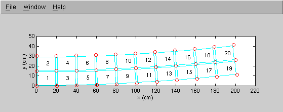
Figure 3 shows the cantilever beam after the displacements have been amplified by a factor of 1000.

The block of code:
    scale = 1000.0;
    for (ii = 1; ii <= 33; ii = ii + 1 ) {
         coord     = GetCoord([ii]);
         nodal_dof = GetDof([ii]);

         if( nodal_dof[1][1] > 0 ) {
             coord[1][1] = coord[1][1] + scale*displ[ nodal_dof[1][1] ][1];
         }
         if( nodal_dof[1][2] > 0 ) {
             coord[1][2] = coord[1][2] + scale*displ[ nodal_dof[1][2] ][1];
         }

         print ii, coord[1][1], coord[1][2], "\n";
    }
systematically retrieves the nodal coordinates and d.o.f. associated with each node from the Aladdin database, and then computes the absolute coordinate of the node after the displacements have been scaled by 1000. The abbreviated output from this block is:
     1          0 cm          0 cm
     2          0 cm      14.98 cm
     3          0 cm         30 cm
     4      20.17 cm     0.1113 cm
     5         20 cm      15.09 cm

    .... details removed .....

    30      178.5 cm      39.02 cm
    31      201.7 cm      11.13 cm
    32        200 cm      26.11 cm
    33      198.3 cm      41.13 cm
This array contains the nodal coordinates used to plot Figure 3.
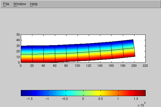
Figure 4 shows the distribution of stresses in the horizontal direction throughout the cantilever beam.

We can use elementary beam theory to verify the accuracy of the results. Assuming that the applied moment is
M = 10 kN x 0.3 m.
and that the beam inertia
I = 1/12 * (0.3 m)^3
it follows that the maximum/minimum stresses are:
stress = M.y_max/I = 2.0 x 10^5 Pa.
which is in the ball-park of stresses for dark blue/red shown along along top/bottom fibers of Figure 4. (Actually, the extrapolated stresses are 1.77 x 10^5 Pa).
Extrapolation of Stresses to Nodal Coordinates
By default the isoparametric plane-strain/plane-stress element will compute and print stress components at the gaussian points of integration. This is where evaluation of the stresses is most accurate.
The block of code:
   M = Zero([4,4]);
   M[1][1] = (sqrt(3) + 1)^2;
   M[1][2] = 2;
   M[1][3] = (sqrt(3) - 1)^2;
   M[1][4] = 2;
   M[2][1] = 2;
   M[2][2] = (sqrt(3) + 1)^2;
   M[2][3] = 2;
   M[2][4] = (sqrt(3) - 1)^2;
   M[3][1] = (sqrt(3) - 1)^2;
   M[3][2] = 2;
   M[3][3] = (sqrt(3) + 1)^2;
   M[3][4] = 2;
   M[4][1] = 2;
   M[4][2] = (sqrt(3) - 1)^2;
   M[4][3] = 2;
   M[4][4] = (sqrt(3) + 1)^2;
   T = Inverse((1/12)*M);
sets up a (4x4) transformation matrix T that will extrapolate stresses at the 4 internal gauss points out to the nodal coordinates. With the matrix T in place, we can now systematically use
actions = GetStress( [ii], displ );
to retrieve the stresses for element "ii" and then compute
and print the "approximate" stresses at the nodal coordinates.
The complete block of code is:
   print "\n";
   print "Element Stresses (sigma_xx at the nodal points)\n";
   print "===============================================\n\n";

   for( ii = 1; ii <= 20; ii = ii + 1 ) {

        /* retrieve stresses and extrapolate out to nodal coordinates    */

        actions = GetStress( [ii], displ );
        extrap  = T*[ actions[1][3];
                      actions[2][3];
                      actions[3][3];
                      actions[4][3] ];

        /* map extrapolated stresses onto nodal coordinate system    */

        extrap = [ 0, 0, 1, 0;
                   0, 0, 0, 1;
                   1, 0, 0, 0;
                   0, 1, 0, 0 ] * extrap;

        /* print extrapolated stresses in format for MATLAB plotting */

        print ii;
        print QDimenLess(extrap[1][1]);
        print QDimenLess(extrap[2][1]);
        print QDimenLess(extrap[3][1]);
        print QDimenLess(extrap[4][1]);
        print "\n";
   }
An unexpected problem we encountered with this method is the mismatch in ordering of the element nodes and gauss integration points. The four-by-four matrix of zeros and ones simply reorders the extrapolated stresses so that they match the nodal points.
The abbreviated output from this block of code is:
      1  1.774e+05  1.774e+05 -1.043e+04 -1.043e+04
      2  1.043e+04  1.043e+04 -1.774e+05 -1.774e+05
      3  1.774e+05  1.774e+05 -1.043e+04 -1.043e+04
      4  1.043e+04  1.043e+04 -1.774e+05 -1.774e+05

     .... details removed .....

     18  1.043e+04  1.043e+04 -1.774e+05 -1.774e+05
     19  1.774e+05  1.774e+05 -1.043e+04 -1.043e+04
     20  1.043e+04  1.043e+04 -1.774e+05 -1.774e+05
These are the stresses plotted in Figure 4.