In 2022, the artificial intelligence research and deployment company OpenAI, introduced a conversational “large-language” model called ChatGPT, which they had trained on billions of pages of text, almost every book ever published, all of Wikipedia, and selected websites. (You can try it for no cost at https://chat.openai.com/.) The current version, as of late 2025, is ChatGPT-5. There are now many other competing chatbots, such as Google’s Gemini, Microsoft’s CoPilot, Perplexity, Anthropic’s Claude, and most recently, DeepSeek.

 

The strength of chatbots is in language interpretation and writing. For example, chatbots are quite good at tasks like suggesting possible titles for papers, talks, or proposals that you are working on. Just feed it all or a portion of what you have written. They can also paraphrase and outline, which can be useful for writing condensed summaries or abstracts. Chatbots can offer opinions and suggestions as to whether your writing is suitable for a particular audience and will offer to re-write the whole thing, for example to make it more formal or less formal. Their knowledge base is extraordinarily wide and they can often answer very specific questions about technical topics. They are often better than search engines at answering very specific questions about hardware or software programs that would otherwise force you to plow through pages and pages of documentation. They can even write a first draft based on a general description, to help you get started. (For example, the table on page 462 was written by ChatGPT-5).

AI as a programmer’s assistant.

But AIs can go well beyond human language tasks; they can also write code in several computer languages commonly used by scientists, such Matlab, Python, Mathematica, C/C++, R, Pascal, Fortran, HTML, JavaScript, Excel macros, etc. But the critical question is: Can AIs write code easier, quicker, and more accurately that a human, specifically a human who is a busy scientist, not a trained computer programmer?

 

Based on my testing, chatbots can generate working code in Matlab or Python for quite a range of signal processing applications, if you describe the task adequately. I found that they could write code that works for many basic signal processing tasks, if the description is sufficiently complete. But for more complex tasks, its code might not work at all or might not do what you expect. Most often, the cause of failure is that I have written the prompt unclearly or incompletely. It’s somewhat misleading that, even in cases where a chatbot’s code does not work, it is presented in good style, divided into clearly identified sections, usually with explanatory comments for each line, appropriate indentation, examples of use, and even warning that the code may fail under certain circumstances (e.g., division by zero, etc.). There are even AI services that support code development, which currently include GitHub Copilot, Amazon CodeWhisperer, Codex, Tabnine, and even Cursor, Replit, Bolt, and Lovable. Here I will focus on general-purpose chatbots such as ChatGPT, which has a feature called “Canvas” that integrates chat and code editing for Python and other text-based formats (page 456).

 

It's a good idea to start simple and work up. A simple example where chatbots work perfectly is Caruana's Algorithm (page 174), which is a fast way to estimate the parameters of a signal peak that is locally Gaussian near its maximum. I asked the chatbots to create a function that

“accepts two vectors x and y approximating a digitally sampled peak, takes the natural log of y, fits a parabola to the resulting data, then computes the position, FWHM, and height of the Gaussian from the coefficients of the parabolic fit”.

 

In this case the chatbot does all the required algebra and creates code that is functionally identical to my hand-coded version. Chatbots can be very handy for creating code and graphic illustrations for instructional materials. For example, I asked both ChatGPT and Microsoft’s CoPilot to:

 

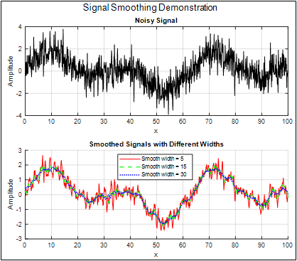
“Write a Matlab script that creates a plot with two horizontal subplots, the top one showing a signal with several peaks and some random noise, and the bottom one showing the results of applying a smooth of three different widths to that signal, each shown in a different line style and color, with a legend identifying each plot and its smooth width”.

This results in a script that generates the graphic shown here, just as requested, although CoPilot included only one of the smooth widths in its legend. (Note that the chatbots are forced to make choices for several things that I did not specify exactly, including the shape of the peaks, the sampling rate and signal length, and the three smooth widths. Moreover, it adds titles to both subplots, even though I did not specify that detail). 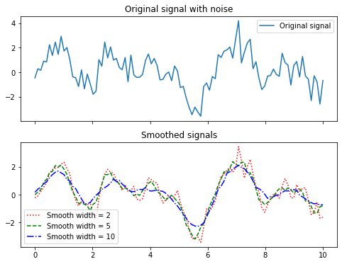It is particularly handy that, if you want to generate a Python equivalent for example, you can simply say “How can I do that in Python” and it creates a working python script that imports the required libraries and generates an almost identical graphic. Although in this case it chose a much lower sampling rate. (The same may be true of the other languages that it knows, but I have not tested that). You can also feed it a program written in one of its languages and ask it to convert it into another of its languages. Sometimes the code generated by chatbots will result in an error, notated by a red warning message in the console of both Matlab and Python/Spyder. You can just copy that error message and paste it directly into the chatbot and it will attempt to fix the problem, often successfully.

 

Another query that created well-structured, easily-modified, 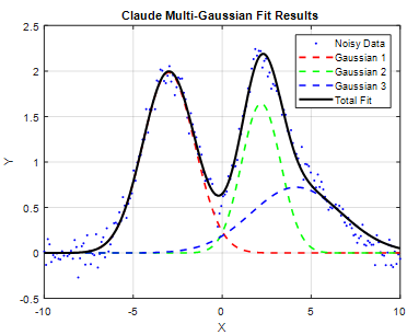functional code is

 

“Create a function that fits the sum of n Gaussian functions to the data in x and y, given the value of n and initial estimates of the positions and widths of each Gaussian, then repeats the fit 10 times with slightly different values of the initial estimates, takes the one with the lowest fitting error and returns its values for the position, width, and height of all the best-fit Gaussians”.

 

ChatGPT and Claude produce code that works and, without me even asking, creates a script that demonstrates it with a nice graph. Other cases where chatbot code worked well:

 

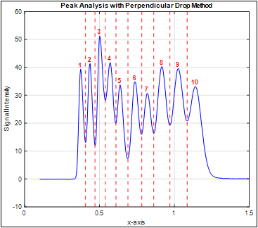
“Create a function that accepts a signal (x,y), then applies the perpendicular drop method to measure the peak widths. Plot the test signal and draw the vertical lines at each minimum.”

 

Both ChatGPT and Claude managed this neatly, as shown in the graphic below.

 

Other examples include:

·       creating a Kalman filter,

·       demonstrating the bootstrap method,

·       detecting peaks and estimating their areas by perpendicular drop (shown on the right),

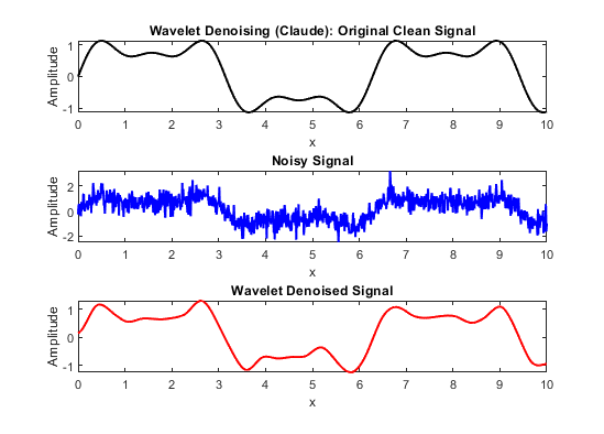
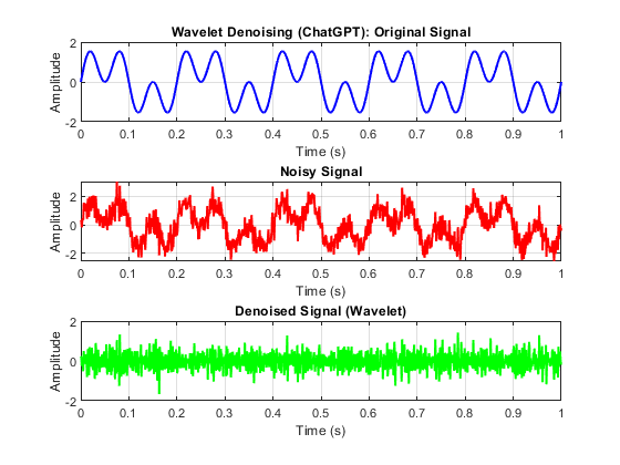
·       demonstrating wavelet denoising (for which Claude’s version worked better that ChatGPT’s),

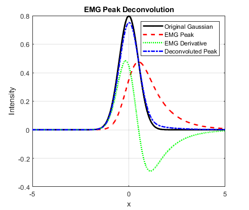
·       and creating a function that symmetrizes exponentially broadened peaks by first-derivative addition, where Claude worked better than ChatGPT, Gemini, or Perplexity (graphic).

 

 

Clearly asking a chatbot to perform routine tasks such as these is quick and convenient, especially if you are creating the equivalent code in more than one language; it spits out the code faster than I can type. For larger more complex projects, you could break up the code into smaller chunks or functions that a chatbot can handle separately and that you can test separately, then combine them later as needed.

 

A chatbot  always presents its results nicely formatted, with correct spelling and grammar, which many people interpret as a “confident attitude”. This inspires trust in the results, but just as for people, being confident does not always mean being correct. There are several important caveats:

 

First, the code that a chatbot generates is not necessarily unique; if you ask it to repeat the task, you’ll sometimes get different code (unless the task is so simple that there is only one possible way to do it correctly). This is not necessarily a flaw; there is often more than one way to code a function for a particular purpose. If the code requires variables to be defined, the names of those variables will be chosen by a chatbot  and won’t always be the same from trial to trial. Moreover, unless you specify the name of the function itself, a chatbot  will choose that name as well, based on what the function does). 

 

Second, and more importantly, there may be more than one way to interpret your request, unless you have very carefully worded it to be unambiguous. Take the example of data smoothing (page 42). On the face of it, this is a simple process. Suppose you ask for a function that performs a sliding average smooth of width n and applies it m times. How will that request be interpreted? If you simply say

 

“…apply an n-point sliding average smooth to the y data and repeats it m times",

 

you will get this code, which does what you asked but probably not what you want. The point of applying repeat smooths is to apply the smooth again to the previously smoothed data, not to the original data, as this code does. The general rule is that n passes of a m-width smooth results in a center-weighted smooth of width n*m-n+1. You will get what you want if you ask ChatGPT for a function that:

“…applies an n-point sliding average smooth to y and then repeats the smooth on the previously smoothed data m times”.

 

This is a small but critical difference, resulting in this code, whereas the previous code returns a singly-smoothed result no matter the value of m.

 

Third, there may be unspecified details or side effects that may require addressing, such as the expectation that the number of data points in the signal after processing should be the same as before processing. In the case of smoothing, for example, there is also the question of what to do about the first n and last n data points, for which there are not enough data points to compute a complete smooth (see page 45). There is also the requirement that the smooth operation should be constructed so that it does not shift the x-axis positions of signal features, which is critical in many scientific applications. Human-coded smooth algorithms, such as fastsmooth, consider all these details.

 

Another example of unspecified details is the measurement of the full width at half-maximum (FWHM) of smooth peaks of any shape. The function I wrote for that task is “halfwidth.m”. I used its description as the ChatGPT query:

 

“…a function that accepts a time series x, y, containing one or more peaks, and computes the full width at half maximum of the of the peak in y nearest xo. If xo is omitted, it computes the halfwidth from the maximum y value”.

 

 

The AI came up with “computeFWHM.m”, which works well if the sampling rate is high enough. However, the AI’s version fails to interpolate between data points when the half-intensity points fall between data points and thus is inaccurate when the sampling rate is low, because I did not specify that it should do so. “CompareFWHM.m” compares both functions on some synthetic data with adjustable sampling rate.

 

Also, chatbots cannot evaluate the graphical results of their calculations. For example, if you ask it to apply some operation, and the graphical result is clearly incorrect, it does not have a clue. But you can complain about that to the chatbot and it will attempt a correction, sometimes successfully.

 

Another technical kink relates to the common Matlab practice of saving functions that you have written as a separate file in the path and then later calling that saved function from a script that you are writing, relying on Matlab to find it in the path. If you ask ChatGPT to convert that new script to another language, you must embed your external functions directly into the code (Matlab R2016b or later).

 

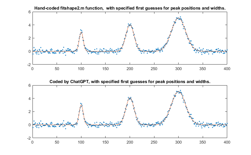
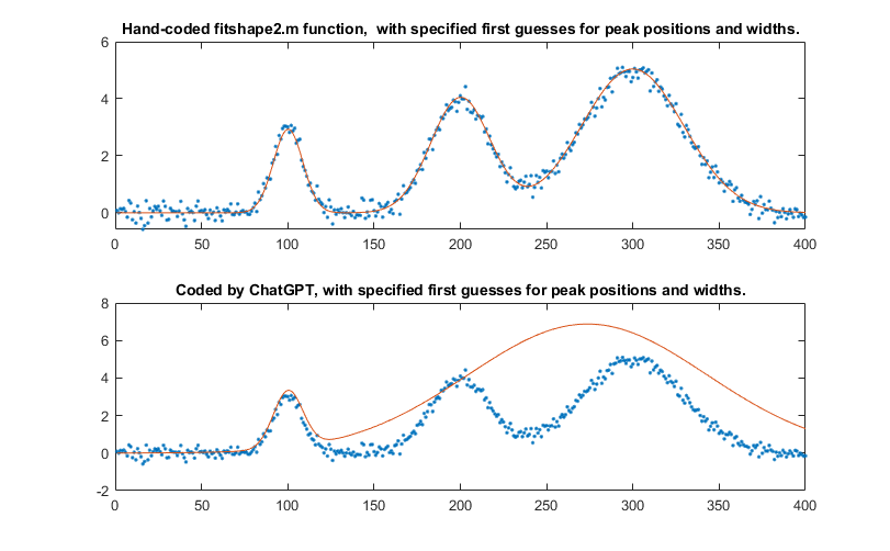
A more challenging signal processing task is iterative fitting of noisy overlapping peaks (page 204). I asked ChatGPT to…

 

“fit the sum of n Gaussian functions to the data in x and y, given initial estimates of the positions and widths of each Gaussian, returning the position, width, and height of all the best-fit Gaussians”.

 

ChatGPT came up with the attractively coded “iterativefitGaussians.m”. The closest hand-coded equivalent in my tool chest was fitshape2.m (page 204); both codes work, are about the same length, and require similar input and output arguments. There is seldom a uniquely correct answer to iterative fitting problems, but the difference in performance between these two codes is instructive. The self-contained script “DemoiterativefitGaussians2.m” compares these two functions for a simulated signal with three noisy peaks whose true parameters are set in lines 13-15. For an “easy” test case, with little peak overlap, both codes work well. But if the peaks overlap significantly, ChatGPT’s code fails to yield a good fit but my fitshape2.m code does work. The difference is probably due to the different minimization functions employed (lsqcurvefit.m vs fminsearch.m).

One task that gave the chatbots some trouble was Gaussian Fourier self-deconvolution (page 114). After several attempts at writing prompts, ChatGPT did the job with the prompt:

 

“Matlab function that performs Fourier self-deconvolution as a means for sharpening the width of signal peaks in x,y, by computing the Fourier transform of the original signal, dividing that by the Fourier transform of a zero-centered Gaussian function of width deconvwidth, performing an inverse Fourier transform of the result, and applies a smoothing function of width smoothwidth to the deconvoluted result”.

(Matlab code. Python code)

 

Segmented processing functions, treated on page 333, are very useful in cases where the signal varies in character along its length so that a single processing function setting is not optimum. Basically, the idea is that you break up the signal into segments, process each segment with different settings, then reassemble the processed segments. A simple example is segmented smoothing (page 55). In the signal shown in blue, below left, the peaks increase in width as x increases, a smaller smooth width should be applied to the early peaks to prevent peak distortion. The following prompt seemed reasonable:

 

“Write a function that accepts a signal vector y and a vector s of length n, makes n copies of y, smooths each one with a smooth width equal to the n^th element of the vector s, then reassembles the smoothed signal from the n^th segment of the n^th copy.”

 

But when the resulting function is applied to the signal in blue on the left, the smoothed signal, in red, exhibits serious discontinuities. The problem is caused by the “end effects” of smoothing, described on  page 45. I then tried writing a more explicit and lengthy description:

 

 “Write a function that accepts a signal vector y, a number of  segments n, an initial smooth width Wstart and a final smooth width of Wend, creates vector S of length n, whose first element is Wstart, last element is Wend, and the other elements are evenly distributed between Wstart and Wend. The function makes n copies of y, smooths each one with a smooth width equal to the n^th element of the vector S, then reassembles the smoothed signal from the n^th segment of the n^th copy”.  The result is shown on the left.

For more complex functions, it rapidly gets to the point where it’s impossible to completely describe the function in enough detail. This is especially true of open-source code that has been developed incrementally over time, with lots of added options and features suggested by many users, such as my 5500-line interactive peak fitter, ipf.m (page 417), or my 4000-line peakfit.m function (page 397) which takes up to 12 input arguments, provides 8 output values, and fits 50 different peak shapes. Even describing such functions completely for a chatbot would be tedious at best. It’s unrealistic to expect any chatbot to completely replace such efforts.

 

ChatGPT cannot write Matlab Live Scripts or Apps because they are not text files. (In contrast, chatbots can write GUI applications in Python. See page 454). However, you can easily convert a chatbot-generated Matlab script into a Live Script, as described on page 368, or you can have chatbots write keyboard-controlled interactive functions, like those described on page 397. I tested this idea with a simple pan-zoom-smooth function, using the prompt:

 

“Write a Matlab function that accepts and plots a signal as an x,y pair and has pan and zoom functions that are interactively controlled by the keyboard cursor keys, using the left and right cursor keys to pan back and forth and the up and down keys to zoom in and out. Add a smoothing function that uses the A and Z keys to increase and decrease the smooth width.”

 

Oddly, ChatGPT and Claude failed with the zoom part of this function, for reasons that are not clear, but Perplexity succeeded. This code could serve as the bones of a customized interactive function with your own additional keypress functions added. This approach, while primitive by GUI standards, is easy to program and can be quite versatile, considering the large number of keys available on a standard keyboard (with and without the Shift key pressed). It also has the advantage that screen space is not occupied by GUI widgets. See page 506 for examples of such keystroke-driven applications.

 

A lot of thought and experience goes into hand-coded programs. An experienced human coder knows the typical range of applications and anticipates typical problems and limitations, especially as those apply to the specific field of applications, such as signals generated by different types of scientific instrumentation. Of course, AIs do know a great deal about specific computer languages and their capabilities and inbuilt functions, which can be very useful, especially if you are re-coding an algorithm in a new or less familiar computer language. But AIs are no replacement for human experience. It goes without saying that you must test any code that a chatbot gives you, just as you must test your own code.

 

I recommend that you be bold and optimistic when exploring the coding abilities of AIs. Ask them to do more than you think they should be able to do; you may be surprised. There is no (or little) cost involved, and AIs are completely non-judgmental and totally tireless. The results you get may not work exactly as you wish, but every failure is a learning opportunity, and you can simply explain the nature of the failure to the AI and it will attempt to correct it. Even if it takes several trials to get it right, the whole process will probably be faster than writing all the code yourself. In addition, you can learn quite a bit by inspecting the code that it generates and the functions and imported modules that it employs. For example, you can use AIs to develop Graphic User Interface (GUI) applications in Python (page 454) or in Mathematica (page 462).

 

Python: free, open-source and powerful

 A popular alternative to Matlab for scientific programming is Python, which is a free and open-source language, whereas Matlab is closed, proprietary, and can be costly. The two languages are different in many ways, and an experienced Matlab programmer might have some difficulty converting to Python, and vice versa, but chatbots can help you, both in setting up a suitable Python environment and in writing code (page 442). Anything that I have done in this book using Matlab, you can do in Python. I do not intend to provide a complete introduction to Python, any more than I did for Matlab or for spreadsheets, because there are many good online sources. Rather, I will review a few of the crucial computational methods, showing how to do the calculations in Python and compare the code side-by-side to the equivalent calculation in Matlab. In addition, I will compare the execution times of both, running on the same desktop computer system, to see if there is any advantage in execution speed or code size one way or the other. For these tests, I was running Python 3.8.8; Anaconda Individual Edition 2020.11, using the included Spyder 5.0.5 desktop (screen graphic), and Matlab 2021: 9.10.0.1602886 (R2021a), both running on a Dell XPS i7 3.5Ghz tower. Both Matlab and Python/Spyder have an integrated editor, code analysis, debugging, ability to edit variables, etc.

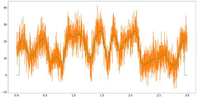
Sliding average signal smoothing

(Based on  Nita Ghosh’s Scientific data analysis with Python: Part 1 )

A “sliding average” smooth is simple to implement using the inbuilt “mean” function in both languages.

 

Python

import numpy as np

import matplotlib.pyplot as plt

from pytictoc import TicToc

t = TicToc()

plt.rcParams["font.size"] = 16

plt.rcParams['figure.figsize'] = (20, 10)

sigRate = 1000 #Hz

time = np.arange(0,3, 1/sigRate)

n = len(time)

p = 30 #poles for random interpolation

ampl = np.interp(np.linspace(0,p,n),np.arange(0,p),np.random.rand(p)*30)

noiseamp = 5

noise = noiseamp*np.random.randn(n)

signal = ampl + noise

t.tic() # start clock

plt.plot(time, ampl)

plt.plot(time, signal)

filtSig = np.zeros(n)

k = 50

for i in range(k,n-k-1):

    filtSig[i] = np.mean(signal[i-k:i+k])

plt.plot(time, filtSig)   

t.toc()  # stop clock print time

# Save signal to file

np.savetxt('SlidingAverageSignal.out',(time, signal), delimiter=',')

 

In the first several lines, Python must import some packages that are required for numerical computing; Matlab has much of that built-in, but there are optional add-on “toolboxes” (e.g. page 132). The Python code creates a simulated noisy “signal” in the first block of code and then uses the inbuilt “savetext” function to save it to disc for Matlab to read, ensuring that the exact same signal is used for both.

 

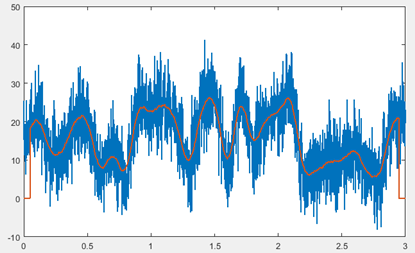
Matlab

clf

load SlidingAverageSignal.out

x=SlidingAverageSignal(1,:);

y=SlidingAverageSignal(2,:);

 

tic % start clock

lx=length(x);

filtsig=zeros(1,lx);

k=50; % smooth width

for i=k:lx-k-1

    filtsig(i)=mean(y(i-k+1:i +k));

end

plot(x,y,'g',x,filtsig,'linewidth',1.5)

toc % stop clock and print elapsed time

 

The fundamental thing here is the use of the “mean” function in both languages to compute the mean of k adjacent points for the smoothed signal.  In Python this is done by the lines:

 

k = 50

for i in range(k,n-k-1):

    filtSig[i] = np.mean(signal[i-k:i+k])

 

and in Matlab by:

 

k=50;

for i=k:lx-k-1

    filtsig(i)=mean(y(i-k+1:i +k));

end

 

You can see how similar they are. (I’ve used the same variable names to make the comparison easier). A key difference is how a block of code is specified, such as a loop or a function definition. In Python, this is done using indentation, which is rigorously enforced. In Matlab, it is done using “end” statements; indentation is optional in Matlab but, as a matter of good coding style, is easily done by the “Smart Indent” in the right-click menu. (See an example of function definition in the iterative least-squares example on page 451). Another important difference: Python uses square brackets to enclose the index to arrays rather that parentheses as does Matlab. Python arrays are indexed from zero; Matlab’s are indexed from 1; so, for example, the first two elements of an array A in Python are A[0] and A[1] but in in Matlab they are A(1) and A(2). Little things mean a lot.

 

To compare the execution times, I have used the “tic” and “toc” statements (inbuilt in Matlab but added to Python by the TicToc package) to start and stop a timer. I have bold-faced those lines in the code, to make it clear that I am counting and timing only the “inner” portion of the code that will have to be repeated if you have multiple data sets to process. I don’t count the time required by the initial set-up, loading of packages, etc. – things that need be done only once. 

 

Python: 8 lines; 0.04 – 0.08 sec

Matlab: 7 lines: 0.007 – 0.008 sec

Both programs are about the same length, but Matlab is clearly faster in this case.

 

Fourier transform and (de)convolution

The Fourier transform (FT) is fundamental for computing frequency spectra, convolutions, and deconvolution. The codes here simply create a vector “a” of random numbers, compute the FT, multiply it by itself, and then inverse FT the result, both using the fft and ifft functions. This is basically a Fourier convolution. Deconvolution would be the same except that the two Fourier transforms would be divided. As before, tic and toc mark the timed blocks.

 

Python:

import numpy as np

from scipy import fft

from pytictoc import TicToc

t = TicToc()

t.tic() # start clock

min_len = 93059  # prime length is the worst case for speed

a = np.random.randn(min_len)

b = fft.fft(a)

c=b*b

d=fft.ifft(c)

t.toc()  # stop clock and print elapsed time

 

 

Matlab:

tic

MinLen = 93059; % prime length is the worst case for speed

a=randn(1,MinLen);

b = fft.fft(a)

c=b.*b;

d=ifft(c);

toc

 

Python: 5 lines; 0.01 – 0.04 sec (The execution time apparently varies with different random number sequences).

Matlab: 5 lines: 0.008 – 0.009 sec

 

 

Classical Least Squares

The Classical Least Squares (CLS) technique has long been used in spectroscopic analysis of mixtures, where the spectra of the individual components are known but which overlap additively in mixtures (page 188). A comparison of Python and Matlab coding for this method is given on page 198. (I wrote the Matlab code first, copied and pasted it into the Spyder editor, and converted it line by line). After the required importation of required Python packages, the codes  (NormalEquationDemo.py and NormalEquationDemo.m) are remarkably similar, differing mainly in the use of indentation, the way functions are defined, the way arrays are indexed, the way vectors are concatenated into matrixes, and the coding of matrix transpose, exponentiation and dot products.

Python: 50 lines; 0.017 sec.  Matlab: 41 lines. 0.018 sec.

Iterative least-squares fitting

(Based on  Chris Ostrouchov’s code on https://chrisostrouchov.com/post/peak_fit_xrd_python/)

 

Python:

import math

import numpy as np

import matplotlib.pyplot as plt

from scipy import optimize

from pytictoc import TicToc

t = TicToc()

def g(x, A, μ, σ):

    return A / (σ * math.sqrt(2 * math.pi)) * np.exp(-(x-μ)**2 / (2*σ**2))

def f(x):

    return np.exp(-(x-2)**2) + np.exp(-(x-6)**2/10) + 1/(x**2 + 1)

A = 100.0 # intensity

μ = 4.0  # mean

σ = 4.0 # peak width

n = 500 # Number of data points in signal

x = np.linspace(-10, 10, n)

y = g(x, A, μ, σ) + np.random.randn(n) 

 

t.tic() # start clock

def cost(parameters):

    g_0 = parameters[:3]

    g_1 = parameters[3:6]

    return np.sum(np.power(g(x, *g_0) + g(x, *g_1) - y, 2)) / len(x)

initial_guess = [5, 10, 4, -5, 10, 4]

result = optimize.minimize(cost, initial_guess)

g_0 = [250.0, 4.0, 5.0]

g_1 = [20.0, -5.0, 1.0]

x = np.linspace(-10, 10, n)

y = g(x, *g_0) + g(x, *g_1) + np.random.randn(n)

fig, ax = plt.subplots()

ax.scatter(x, y, s=1)

ax.plot(x, g(x, *g_0))

ax.plot(x, g(x, *g_1))

ax.plot(x, g(x,*g_0) + g(x,*g_1))

ax.plot(x, y)

t.toc()  # stop clock and print elapsed time

 

np.savetxt('SavedFromPython.out', (x,y), delimiter=',') # Save signal to file

 

Iterative curve fitting is more complex than the previous examples. Both Python and Matlab have optimization functions (“optimize.minimize” in the Python code, above; the inbuilt “fminsearch” in the Matlab code, below). The optimize function in Python is more flexible and can use several different optimization methods. Matlab uses the Nelder-Mead method, which is used below (see page 204), but there is also an optional optimization toolbox that provides alternative methods if needed.

 

clear

clf

load SavedFromPython.out

x=SavedFromPython(1,:);

y=SavedFromPython(2,:);

start=[-5 3 6 3];

format compact

global PEAKHEIGHTS

tic

FitResults=fminsearch(@(lambda)(fitfunction(lambda,x,y)),start);

NumPeaks=round(length(start)./2);

for m=1:NumPeaks

  A(m,:)=shapefunction(x,FitResults(2*m-1),FitResults(2*m));

end

model=PEAKHEIGHTS'*A;

plot(x,y,'- r',x,model)

hold on;

for m=1:NumPeaks

    plot(x,A(m,:)*PEAKHEIGHTS(m));

end

hold off

toc % stop clock and print elapsed time

function err = fitfunction(lambda,t,y)

global PEAKHEIGHTS

A = zeros(length(t),round(length(lambda)/2));

  for j = 1:length(lambda)/2

     A(:,j) = shapefunction(t,lambda(2*j-1),lambda(2*j))';

  end

PEAKHEIGHTS = A\y';

z = A*PEAKHEIGHTS;

err = norm(z-y');

end

function g = shapefunction(x,a,b)

g = exp(-((x-a)./(0.6005612.*b)) .^2); % Expression for peak shape

end

 

Python: 16 lines; 0.02-0.08 sec

Matlab: 25 lines; 0.01-0.03 sec

 

The Matlab algorithm here is the same as used by my peakfit.m (page 396) and ipf.m (page 417) functions. The elapsed times of both Matlab and Python vary with the random noise sample, but in this example, Matlab has an advantage in computational speed, which might be significant some applications.

 

An excellent step-by-step introduction to iterative curve fitting in Python is by Emily Grace Ripka.

Peak Detection

 The automatic detection of peaks is a common requirement. The coding required is a little more complex. The codes are based on the Python example in the SciPy documentation: https://docs.scipy.org/doc/scipy/reference/generated/scipy.signal.find_peaks.html. Both languages have a “find peaks” function, but Matlab’s function is rather slow, so I prefer to code my own algorithm in Matlab using nested loops (each with an “end” statement but also indented for clarity). The signal used here is a portion of an electrocardiogram that is included as a sample signal in Python. The task is to detect the peaks that exceed a specified amplitude threshold and mark them with a red “x” on the plot.

 

Python:

import numpy as np

import matplotlib.pyplot as plt

from scipy.misc import electrocardiogram

from scipy.signal import find_peaks

from pytictoc import TicToc

t = TicToc()

x = electrocardiogram()[2000:4000]

t.tic() # start clock

peaks, _ = find_peaks(x, height=0)

plt.plot(x)

plt.plot(peaks, x[peaks], "x")

plt.plot(np.zeros_like(x), "--", color="gray")

plt.show()

t.toc()  # stop clock and print elapsed time

np.savetxt('FindPeaks.out',(x), delimiter=',')

Matlab:

load electrocardiogram.out;

y=electrocardiogram;

tic % start clock

  plot(1:length(y),y,'-k')

  height=0;

  x=1:length(y);

  peak=0;

  for k = 2:length(x)-1

      if y(k) > y(k-1)

          if y(k) > y(k+1)

              if y(k)>height

                  peak = peak + 1;

                  P(peak,:)=[x(k) y(

k)];

              end

          end

      end

  end

  hold on

  for k=1:length(P)

      text(P(k,1)-12,P(k,2),'x','color',[1 0 0])

  end

  grid

  hold off

toc % stop clock and print elapsed time

 

Python: 5 lines; 0.01  sec

Matlab: 19 lines: 0.007 sec as written (1.5 sec using the Matlab inbuilt findpeaks.m function)

Here, the advantage goes to Python, because its inbuilt “findpeaks” function is superior to Matlab’s.

 

The bottom line

On average, Matlab is slightly faster for most of these signal processing applications, but that advantage could easily be outweighed by the fact that Python is free and open-source, which is a strong argument in its favor. (And Python is certainly faster than the free Matlab clone Octave). I would recommend this: if you have a background in computer science or have taken some courses, then you will probably prefer Python. Others might find Matlab easier to work with. I like both languages, but I have mainly used Matlab, because it has so many well-developed toolboxes and because it acts and feels more finished and polished than either Anaconda/Python/Spyder or the Matlab clone Octave, in my opinion. After all, Mathworks Inc has remained in business selling the very costly Matlab, while Python is free. There must be a reason. (As of 2023, over 2,200 universities worldwide have a Campus-Wide License for MATLAB and Simulink).

 

Using AI to develop Graphic User Interface applications in Python.

 

While Matlab has a GUI development environment for Matlab Apps (page 370), the process is complex and, because it is not text-based, cannot be coded by a chatbot. Python has several libraries for creating GUI apps for various purposes, but again the details can be complex and it is arguably easier to describe the desired functionality to a chatbot and to have it write the code and handle all the messy details. The fully functional example on the right was created by this remarkably short prompt:

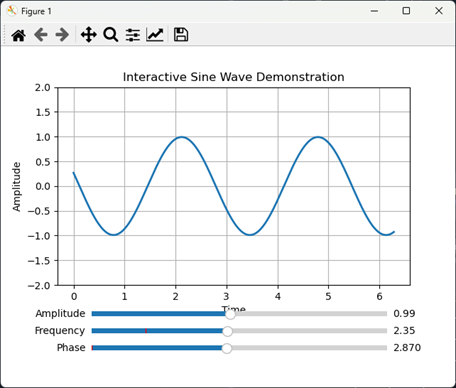
“Write a python script that creates an interactive demonstration of the properties of a sine wave, with three sliders to demonstrate the amplitude, frequency, and phase”.

 

The Python code is only 58 lines. In this case I allowed ChatGPT to choose the GUI library and to design the layout. It chose “matplotlib”, a popular Python library for creating static, animated, and interactive visualizations that is widely used in data analysis and scientific computing.

 

But matplotlib is not without problems. Its “widgets” (sliders, radio buttons, etc.) can sometimes be finicky in certain environments, especially when running inside IDEs like Spyder. Fortunately, Python has more robust GUI libraries like PyQt5 and Tkinter, which are a better solution for creating interactive applications.

 

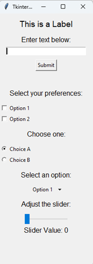
I asked ChatGPT to “create a simple demonstration of the main Tkinter widgets. The result is shown on the left, including:

 

1. Label: Displays static text.
2. Entry: A single-line text box.
3. Button: Performs an action when clicked.
4. Checkbox: Allows multiple selections.
5. Radio Button: Allows a single selection from multiple options.
6. Dropdown Menu: Lets the user choose from a predefined list.
7. Slider: Adjusts the value of a variable by sliding.
8. Dynamic Updates: Text and slider values are updated interactively.
   
   This, plus its ability to handle mouse motions and buttons, seems to cover most of the GUI widgets one is likely to need for signal processing applications.

 

 

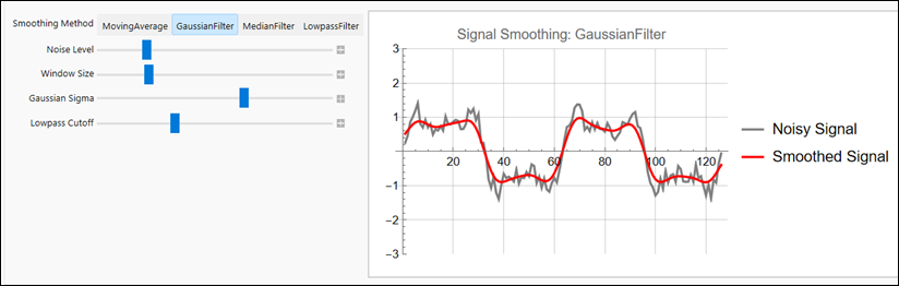
For a more practical signal processing application, I asked ChatGPT to create a Python GUI data smoothing tool that:

 

“… has an Open File button that opens a file browser, allowing you to navigate to your data file (in .csv or .xlsx format; assume that the x,y data are in the first two columns) and a Save File button for saving the smoothed result. Plot the original signal in black and the smoothed result in red. Add a SmoothType drop-down menu that selects the smoothing algorithm. The first choice in that menu is a multi-pass sliding average smooth. Add two sliders, the first that controls the smooth width (from 3 points to 10% of the number of points in the data) and the second that controls the number of passes of the sliding average (1-5 passes). The second item in the SmoothType menu should be the Savitsky-Golay smooth, with two sliders to control the frame length and polynomial order of the smooth. Allow the user to zoom in and out to inspect details the signals using the mouse wheel to expand or contract the x-axis range. Use the mouse left-button drag to pan back and forth. Update the plot for each change in any of the controls.”

 

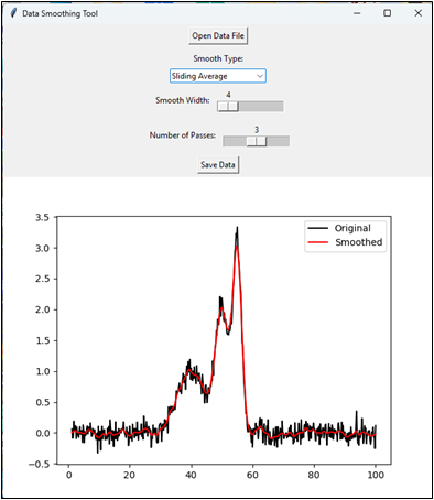It took only a minute for the AI to generate this 198-line solution, quicker that most people can type. The Python code uses the Tkinter, matplotlib, pandas, and scipy libraries. It runs without trouble in the Spyder IDE or directly from the Anaconda PowerShell prompt window. Even if it does not look or behave like you wanted, you can just ask to add or change those aspects and the AI will do it.

 

 Clearly this could be expanded as needed for many signal-processing purposes, along the lines of the Matlab Live Scripts described on page 369.

The example on the right below is an AI-written tool for Gaussian Fourier self-deconvolution (page 117), with sliders to control the width of the Gaussian deconvolution function and the cutoff frequency and rate of the Fourier filter Python script. Data file.

 

Python’s GUI apps like this are more versatile and are better at isolating the user interface from the code. (Matlab Live Scripts imbed the GUI controllers directly in the code, which is very convenient for rapid coding and prototyping, but it also makes the code vulnerable to accidental modification if the scripts are used by inexperienced users).

ChatGPT + Python

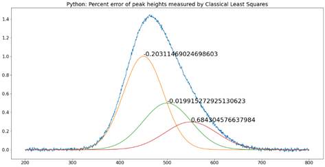
When you are working with coding, specifically Python coding, ChatGPT has two modes of operation: Chat mode and Canvas mode, which is optimized for code generation and testing. Chat Mode is the default; in that mode everything stays in a single conversation flow in a large browser window, with code, discussions, tables, and graphic visualizations. You can expand or download the graphics or change the colors of the lines interactively. (As always, a scrolling list of other chats is on the left). This mode is good for iteratively testing small changes and for back-and-forth problem-solving. If requested, it will display the code it uses and you can copy and paste that into Spyder or into a Note and save it as a “.py” file and run it from the command window. (ChatGPT can write code in Matlab as well but cannot execute it. You must copy and paste the code into Matlab’s editor window).

 

 

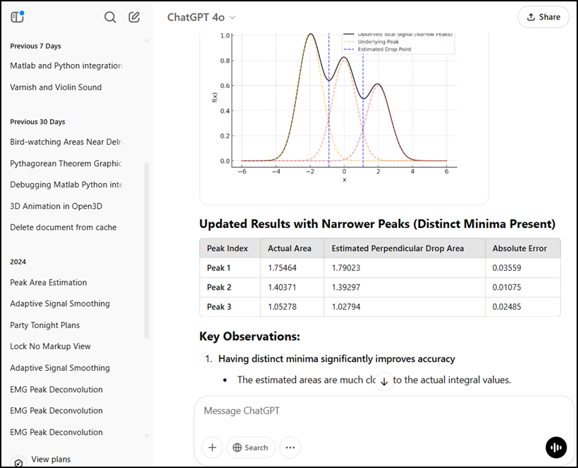
In the example shown above, I asked ChatGPT to “prepare a graphic example of the perpendicular drop method of estimating the areas of overlapping peaks”. (Interestingly, it “cheated” in its first attempt and used its prior knowledge of the individual peak parameters. Once I pointed that out, it used a properly data-driven approach. Artificial intelligence only goes so far. Always be skeptical). You can ask for other changes, such as different peak shapes, heights, and widths, greater or less peak separation, noise added to the original signal, or you can ask it to display the peak area errors as percentages in the table.

In Canvas Mode the code is kept in a dedicated editor window where you collaboratively edit code or text files. It provides versioning options, such as "Show changes" and "Previous version", so you can track edits and revert to earlier versions of code if needed. You can make changes, ask questions, and request modifications, all while seeing the current document content in real time. You can return the Chat Mode simply by refreshing the browser.

 

 

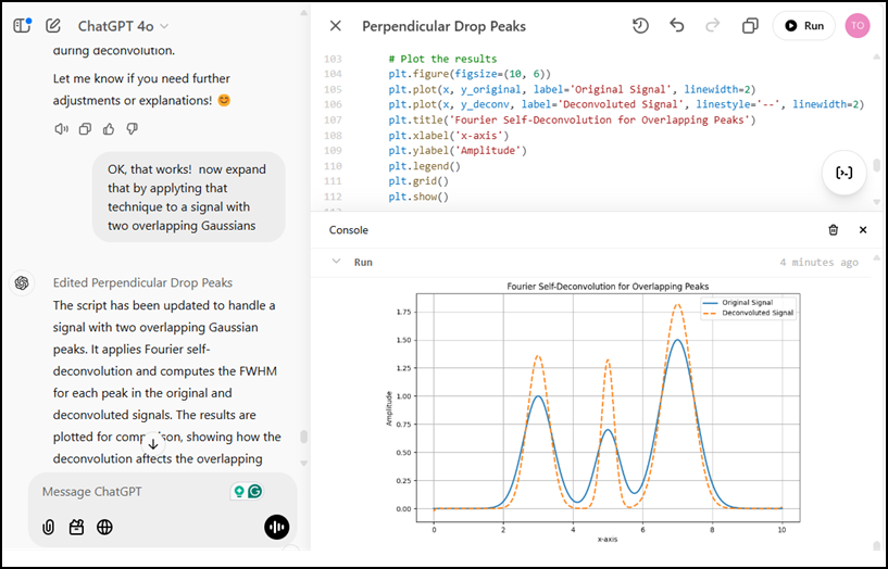
The Canvas mode is shown here by the example of Fourier self-deconvolution. The left-hand panel shows a portion of the chat conversation. When you click the Opens Canvas button in the upper right of the browser window, it displays the code that it creates in that panel. You can ask for any type of calculation, simulation, with tabular or graphical output. The text and graphic outputs are displayed in the lower right Console. You can ask ChatGPT for additions or modifications and the code will be corrected. Buttons allow you to revert to the previous version, fix bugs, copy the code for pasting elsewhere, port to C++, Java, JavaScript, TypeScript, etc. If an error pops up, click on it to have the AI attempt a correction. (Unfortunately, within the Canvas environment, you cannot directly execute code that requires external libraries like Tkinter to install or set up, but you can copy and paste the code into Python’s editor).

 

Formats supported by Canvas include Python, C/C, Java , JavaScript, HTML/CSS, JSON/XML, and Markdown. See https://openai.com/index/introducing-canvas/

 

Chatbots are developing rapidly as I write this in late 2025. By the time you read this, they will certainly have added new features and capabilities.

Connecting Matlab and Python

Up to now, I have considered Matlab and Python as separate islands, but here you will learn how to connect them, enabling the integration of Matlab's powerful numerical capabilities with Python's vast libraries and flexibility. This can be useful in both directions. For example, from Matlab you can call those Python GUI applications that were so easily developed using ChatGPT to write the code (page 454). And from Python, you can call any of the Matlab functions in the Matlab File Exchange or even those that I have developed (page 479), such as the peak fitting functions peakfit.m (page 397) and its interactive cousin ipf.m (page 417). The following step-by-step guide, tailored for MATLAB users, shows you how to set up Python, install the MATLAB Engine for Python, and use Python to interact with MATLAB. I assume that you have a recent version of Matlab already installed. Note: if you have worked with Python before, it might be advisable to create a virtual environment for experimentation.

 

First, for this purpose, Matlab works only with Python 3.11. Visit https://www.python.org/downloads/ and download Python 3.11. During installation, check the box Add Python to PATH, select Customize Installation and ensure that all features are selected. To verify Installation, open a command prompt or terminal (Type CMD in the search at the bottom) and type:

 

python --version

 

Confirm that the output displays Python 3.11.x.

 

Installing the MATLAB Engine for Python

Open a Command Prompt or terminal. Change to the MATLAB Engine installation directory:

 

cd "C:\Program Files\MATLAB\R2024b\extern\engines\python"

                            Run the following command to install the engine:

 

python -m pip install .

 

You must include the space and the period at the end: they are important.

 

Open the command window and type :

 

python

 

The prompt will change to >>>, indicating that you are in a Python session. Type in these commands into the Notepad and save them as a “.py” file and run it from the command window.

 

import matlab.engine

eng = matlab.engine.start_matlab()

print("MATLAB is running!")

eng.quit()

If MATLAB starts successfully and displays "MATLAB is running!”, the installation is complete.

 

Examples of calling MATLAB from Python

Here’s a simple example that calls Matlab’s built-in square root function (sqrt) from Python. In the command window, type python and execute the following code:

eng = matlab.engine.start_matlab()

result = eng.sqrt(16.0)

print("Square root:", result)

eng.quit()

 

The result is printed out in the command window.

Square root: 4.0

(The slight delay before printing out the result is normal). You can also execute previously-developed MATLAB functions saved as “.m” files directly from Python. As a simple example, suppose you have defined a Matlab function called “magnitude” and saved it in the current path:

 

function result=magnitude(a,b)

   result=sqrt(a^2+b^2);

end

Now you just replace result=eng.sqrt(16.0)in the previous example with result=eng.magnitude(3, 5). Run the modified script in Python and the results will be printed out as before: 5.8310.

 

Of course, you can call functions that are much more useful than those trivial examples. Here are two examples. The first calls my 4000-line Matlab peakfit.m function (page 397). The Python script is CallpeakfitDemo.py, located in the path: C:\Users\Name\Dropbox\SPECTRUM
where “Name” is your username. The script creates a test signal consisting of two over-lapping Gaussian bands, adds some noise, calls my peakfit.m function, passes the x,y signal vectors, the number of  peaks and the peak shape to that function, which performs an iterative least-squares fit, prints out the best-fit results in the command window, and displays the Matlab figure in a separate window. (The figure is a standard Matlab figure window, which means that it can be resized, the labels can be edited, and it can be saved in multiple formats).

 

There are two ways to call this function from the command window. You can change the current path:

 

C:\Users\Name\Dropbox\SPECTRUM>python CallpeakfitDemo.py

 

or specify the path when you call the function:

 

C:\Users\Name>python C:\Users\Name\FunctionsDirectory\CallpeakfitDemo.py

 

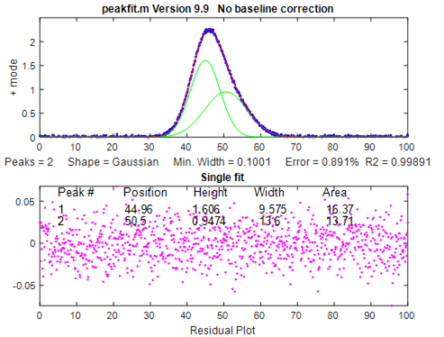
In addition to the graph shown above, the script also prints out the fit results and “goodness of fit” measures in tabular form in the command window:

Peak #  Position    Height      Width       Area

--------------------------------------------------------

1       44.96       1.606       9.575       16.37

2       50.5        0.9474      13.6        13.71

 

Goodness of Fit:

% Fitting Error   R-squared

------------------------------

0.8915            0.9989

(Note: there will be a delay of about 2 seconds before the graph and printout is displayed).

 

The second example is more interactive: CallipfDemo.py, which is also in the same directory. This script creates a test signal consisting of three overlapping Lorentzian bands, adding some noise, and passes the data to ipf.m, which is my keypress-operated interactive curve fitting explorer. You call it in the same way as above. (C:\Users\Name\Wherever is the path to

 CallipfDemo.py on your computer).

C:\Users\Name\Wherever>python CallifpDemo.py

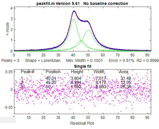(Again, this figure is a standard Matlab figure window, with all its properties). Click on the figure window and use the keypresses to pan and zoom (using the cursor keys), select the desired peak shape (G=Gaussian, L=Lorentzian, etc.), the number of peaks in the model (the number keys), the first-guess start positions (press C, then click on the graph for each peak start position), etc. Other keypress commands are documented on page 419.

 

The same technique can be used for my other Matlab keypress operated functions. Just replace ipf.m with iSignal, isignal.m, page 376, for interactive signal exploration, iPeak, ipeak.m, page 255 for interactive peak detection or iFilter, ifilter.m, page 391 for interactive Fourier filtering. (Note: You can download the entire SPECTRUM folder, which contains all those Matlab functions and more, with their documentation, from this link).

 

Calling Python from Matlab is done with the “system” command. From the Matlab command line:

 

system(‘C:\Users\YourUserName\YourScript.py’)

 

For example, you could use this to call any of the Python GUI modules developed on page 454 such as sine.py, DataSmoothingGUI2.py, or GausSelfDconv.py.

Connecting GNU Octave and Python

Matlab is very expensive to purchase, and if your campus or workplace does not have a site license for it, you might be interested in a less expensive route. GNU Octave (page 22) is a possible alternative. It is almost completely compatible with Matlab and it is a free open-source product. The Python library oct2py provides a high-level Python interface to Octave, allowing you to run Octave commands from Python, pass data back and forth, and call Octave functions. In the Command Prompt window:

 

pip install oct2py

 

Then type :

 

python -Xfrozen_modules=off

 

The prompt will change to >>>, indicating that you are in a Python session.

 

>>> import oct2py

>>> oc = oct2py.Oct2Py()

 

Next, try displaying the sum of 2+2:

 

>>> print(oc.eval('disp(2+2)'))

 

Python responds with:

 

4

 

Next, change the path to the location of your Octave functions:

 

>>> oc.eval('addpath(\"C:/Users/UserName/directory\");disp(\"\")')

 

Where “directory” is the name of the folder where the Octave functions that you have written are stored. In the following example, the custom function “magnitude” simply computes the square root of the sum of the squares of  two numbers:

 

>>> print(oc.magnitude(3,5))

 

5.830951894845301

 

So, all you must do is to add the “oc.” in front of the name of any Matlab or Octave function that is in that path.

 

Calling Python from Octave

 

This works exactly the same as in Matlab, using the “system” function. From the Octave command line:

 

system('python myscript.py')

 

For example, you could call the GUI functions sine.py, DataSmoothingGUI2.py, or GausSelfDconv.py.

 

To capture the output of a function:

 

[status, cmdout] = system('python myscript.py'); disp(cmdout);

Mathematica in Signal Processing – A Comparison with MATLAB and Python

Mathematica is a symbolic-numeric computing platform with a tightly integrated notebook interface and its own high-level language. While Matlab and Python are widely used in engineering and scientific computing, Mathematica is less widely used in those domains but it brings unique capabilities, particularly in symbolic computation, rule-based programming, and dynamic interactivity. It was developed by visionary British computer scientist Stephen Wolfram.

Comparison Table

Feature	Mathematica	MATLAB	Python
Language	Wolfram Language (symbolic first)	MATLAB (imperative, array-oriented)	Python with NumPy/SciPy
Symbolic Computation	✅ Native & deep symbolic capabilities	❌ Limited (Symbolic Math Toolbox)	⚠️ SymPy (less integrated)
Numerical Computation	✅ Built-in	✅ Built-in	✅ NumPy/SciPy
Plotting & Visualization	✅ High-level, publication-ready	✅ Strong 2D/3D plotting	✅ Matplotlib, Plotly, etc.
Interactivity	✅ Built-in (Manipulate[])	⚠️ Via GUI tools	⚠️ Via Tkinter/PyQt/etc.
Notebook Interface	✅ Native .nb	✅ Live Scripts (.mlx)	✅ Jupyter Notebooks
Cost / Licensing	Commercial (academic available)	Commercial (academic available)	Open-source (mostly free)
Signal Processing Tools	⚠️ Smaller, symbolic-oriented	✅ Extensive toolboxes	✅ SciPy, PyWavelets
Learning Curve	Steep for programming, shallow for math	Moderate (especially for engineers)	Moderate–steep (depends on libraries)
LaTeX / Docs Integration	✅ Native typesetting	✅ Good formatting	⚠️ Requires plugins

 

Like Matlab and Python, AI chatbots can be used to create Wolfram code, as illustrated in example 2 on the following page.

Unique Strengths of Mathematica for Signal Processing

 

Signals may be captured live from sensors, instruments and data feeds, stored in files and databases and generated from simulated models and processes.
1. Notebook format

Mathematica integrates code and graphics into one document (simple example: code, graphic). Here’s a more elaborate example, demonstrating second-derivative peak sharpening (page 79).

 

2. Symbolic Signal Models

Mathematica excels at creating exact symbolic expressions for transforms and filters. For example:

    FourierTransform[Exp[-a t] UnitStep[t], t, ω]

 

3. Simple dynamic Interactivity:

Mathematica’s clever Manipulate[] function allows you to create real-time demos with sliders, checkboxes, and controls. Here’s an example: a demonstration of different kinds of data smoothing filters. The Wolfram code, the graph, and the interactive controls are all contained within one Mathematica document, similar to a Matlab Live Script (page 369). (Click the “Enable Dynamics” button on the upper right of the Mathematica notebook).

 

 

4. Specify symbolic forms in plain text format and display in traditional form:

 

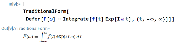
Which is the symbolic form of the Fourier transform.

 

5. Symbolic + Numeric Fusion:

 

You can derive a formula analytically and then apply it numerically. For example, you can derive a symbolic derivative like so:

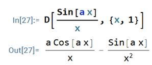
In this code, D is the symbolic derivative: [D[expr, {x, n}] returns the n^th derivative of the expression expr with respect to x). Then you can evaluate that derivative at specific numerical values:

In[28]:= N[D[Sin[a x]/x, x] /. {a -> 2.3, x -> 1.2} ]

 

                    In[29]:= -2.03742
N converts exact/symbolic results to numeric ones.

 

6. Unified Language for Math, Graphics, and GUIs:

 

Mathematica uses one coherent language for symbolic computation, numerical analysis, plotting, and GUI development.

Limitations in Signal Processing Use

• There are fewer built-in signal processing functions compared to MATLAB’s Signal Processing Toolbox or Python’s SciPy.

• There is less widespread use in engineering practice, so fewer textbooks and examples.

• It has a steeper learning curve for procedural programming tasks.

• I have found that data importing in Mathematica is less robust than Matlab’s Import Wizard or Python’s Pandas data analysis package.

Suggested Use Cases in Signal Processing

• Symbolic manipulation of transfer functions

• Interactive educational tools and demonstrations

• Visualizing filter behavior and transforming domains

• Hybrid analytical/numerical derivations

• Related examples: Signal processing, Filter design, Signal analysis, Live playground.

Mathematica may not be the first tool of choice for signal processing implementation, but it excels in theory, visualization, and interactivity. For readers already familiar with MATLAB or Python, Mathematica offers an opportunity to approach signal processing from a more symbolic and exploratory perspective, especially when clarity, derivation, or publication-quality graphics are the goals (true vector graphics, consistent styling via options, precise typography & math, color-blind-safe palettes, and high-quality export).

 

Note: this section was written with the help of ChatGPT5.